View-API for JOOQ Application

August 5, 2018, 1:34 pm

≫ Next: Use the Database as Persistence Layer Only

In this blog post I show how to build a read-only view-API for Oracle’s HR sample schema. And I will use this view-API in a JOOQ application. This application will fully comply with the Pink Database Paradigm (PinkDB). This means the application executes set-based SQL and retrieves data with as few network roundtrips as possible.

The following topics are covered:

This is not meant to be a tutorial. However, you should be able to build the application based on the information in this blog post and the referenced links.

It’s the first time I’ve done anything with JOOQ. I read about it, understood the high-level concepts, but I have never used JOOQ before. This is one reason why this blog post became a bit more verbose. I hope it is helpful.

1. Install Sample Schemas

See the Oracle documentation.

2. Build the View-API

1:1 Views

When building a view API I start with a 1:1 mapping to the table. There are usually some discussions on different topics.

Expose Surrogate Keys

One topic is to include surrogate keys or just business keys in the view-API. Nowadays, I tend to expose surrogate keys. The main reason is to avoid joins when business key columns are stored in related (parent) tables. Forcing the application to join views via such business key columns is a bad idea from a performance point of view.

Convenience Views – Not a Replacement for 1:1 Views

Another topic is the simplification of the model. For example, provide data from various tables to simplify the usage. Simplification means here sparing the consuming application to use joins. This is sometimes a good idea, but it does not replace the 1:1 views, which are the key to the optimal path to the data. I know about join elimination, but in reality they often do not work. One reason is that unnecessary columns are queried as well. Another problem is, to force the view to apply selective predicates as early as possible. Sometimes it is necessary to introduce an application context, just for that purpose, making the usage of the view not that simple anymore.

Value of a 1:1 View-API

The logical next question is this: Why do we need a view layer when it just provides data the same way as the underlying tables? That’s an excellent question. I strongly recommend to introduce a layer only, when it provides more value than the additional effort. So, what is the value of a 1:1 view layer? Most products evolve during their life cycle. Hence, the data model will most probably change as well. When we have a view layer, we have the option to change the physical data model and keep the existing view layer the same for the consuming applications. From that point on, the views are not a 1:1 representation of tables, at least not in every case.

As long as we keep the interface to the application unchanged, we do not have to coordinate changes with the consuming applications. This gives us effectively room for refactoring and simplifies going live scenarios of new releases. Providing additional data and functionality is usually not a problem. But adapting applications to new interfaces needs time. A view-API, especially if it implements some versioning concept, provides an excellent value in this area.

View-API of HR Schema

I’ve generated the initial version of the 1:1 view layer with oddgen‘s 1:1 View generator.

ALTER SESSION SET current_schema=hr;

CREATE OR REPLACE VIEW COUNTRIES_V AS
   SELECT COUNTRY_ID,
          COUNTRY_NAME,
          REGION_ID
     FROM COUNTRIES;

CREATE OR REPLACE VIEW DEPARTMENTS_V AS
   SELECT DEPARTMENT_ID,
          DEPARTMENT_NAME,
          MANAGER_ID,
          LOCATION_ID
     FROM DEPARTMENTS;

CREATE OR REPLACE VIEW EMPLOYEES_V AS
   SELECT EMPLOYEE_ID,
          FIRST_NAME,
          LAST_NAME,
          EMAIL,
          PHONE_NUMBER,
          HIRE_DATE,
          JOB_ID,
          SALARY,
          COMMISSION_PCT,
          MANAGER_ID,
          DEPARTMENT_ID
     FROM EMPLOYEES;

CREATE OR REPLACE VIEW JOB_HISTORY_V AS
   SELECT EMPLOYEE_ID,
          START_DATE,
          END_DATE,
          JOB_ID,
          DEPARTMENT_ID
     FROM JOB_HISTORY;

CREATE OR REPLACE VIEW JOBS_V AS
   SELECT JOB_ID,
          JOB_TITLE,
          MIN_SALARY,
          MAX_SALARY
     FROM JOBS;

CREATE OR REPLACE VIEW LOCATIONS_V AS
   SELECT LOCATION_ID,
          STREET_ADDRESS,
          POSTAL_CODE,
          CITY,
          STATE_PROVINCE,
          COUNTRY_ID
     FROM LOCATIONS;

CREATE OR REPLACE VIEW REGIONS_V AS
   SELECT REGION_ID,
          REGION_NAME
     FROM REGIONS;

View Constraints

When building a view-API it is a good idea to also define primary key, foreign key and unique constraints for these views. They will not be enforced by the Oracle database, but they are an excellent documentation. Furthermore, they will be used by JOOQ as we see later.

ALTER SESSION SET current_schema=hr;

-- primary key and unique constraints
ALTER VIEW countries_v   ADD PRIMARY KEY (country_id)              DISABLE NOVALIDATE;
ALTER VIEW departments_v ADD PRIMARY KEY (department_id)           DISABLE NOVALIDATE;
ALTER VIEW employees_v   ADD PRIMARY KEY (employee_id)             DISABLE NOVALIDATE;
ALTER VIEW employees_v   ADD UNIQUE      (email)                   DISABLE NOVALIDATE;
ALTER VIEW job_history_v ADD PRIMARY KEY (employee_id, start_date) DISABLE NOVALIDATE;
ALTER VIEW jobs_v        ADD PRIMARY KEY (job_id)                  DISABLE NOVALIDATE;
ALTER VIEW locations_v   ADD PRIMARY KEY (location_id)             DISABLE NOVALIDATE;
ALTER VIEW regions_v     ADD PRIMARY KEY (region_id)               DISABLE NOVALIDATE;

-- foreign key constraints
ALTER VIEW countries_v   ADD FOREIGN KEY (region_id)     REFERENCES hr.regions_v     DISABLE NOVALIDATE;
ALTER VIEW departments_v ADD FOREIGN KEY (location_id)   REFERENCES hr.locations_v   DISABLE NOVALIDATE;
ALTER VIEW departments_v ADD FOREIGN KEY (manager_id)    REFERENCES hr.employees_v   DISABLE NOVALIDATE;
ALTER VIEW employees_v   ADD FOREIGN KEY (department_id) REFERENCES hr.departments_v DISABLE NOVALIDATE;
ALTER VIEW employees_v   ADD FOREIGN KEY (job_id)        REFERENCES hr.jobs_v        DISABLE NOVALIDATE;
ALTER VIEW employees_v   ADD FOREIGN KEY (manager_id)    REFERENCES hr.employees_v   DISABLE NOVALIDATE;
ALTER VIEW job_history_v ADD FOREIGN KEY (department_id) REFERENCES hr.departments_v DISABLE NOVALIDATE;
ALTER VIEW job_history_v ADD FOREIGN KEY (employee_id)   REFERENCES hr.employees_v   DISABLE NOVALIDATE;
ALTER VIEW job_history_v ADD FOREIGN KEY (job_id)        REFERENCES hr.jobs_v        DISABLE NOVALIDATE;
ALTER VIEW locations_v   ADD FOREIGN KEY (country_id)    REFERENCES hr.countries_v   DISABLE NOVALIDATE;

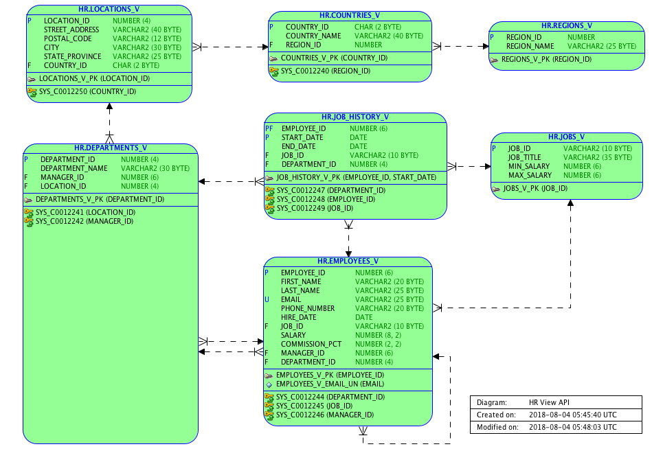
View-API Model

I created the following relational model with Oracle’s SQL Developer. SQL Developer automatically took into account all constraints defined on these 7 views. Most of the work was to rearrange the view boxes on the diagram, but with only 7 views it was no big deal.

3. Create the View-API Database Role

We grant read access to all views as part of the API to the database role HR_API_ROLE. This is easier to maintain, especially when access to more than one connect user is granted.

Please note that just READ access is granted on the views. We do not grant SELECT access to ensure that data can’t be locked by the connect users via SELECT FOR UPDATE. The READ privilege was introduced in Oracle Database 12c.

CREATE ROLE hr_api_role;

GRANT READ ON hr.countries_v   TO hr_api_role;
GRANT READ ON hr.departments_v TO hr_api_role;
GRANT READ ON hr.employees_v   TO hr_api_role;
GRANT READ ON hr.job_history_v TO hr_api_role;
GRANT READ ON hr.jobs_v        TO hr_api_role;
GRANT READ ON hr.locations_v   TO hr_api_role;
GRANT READ ON hr.regions_v     TO hr_api_role;

In this cases it does not make sense to define more than one role. But for larger projects it might make sense to create more roles. For example to distinguish between read and write roles or to manage access to sensitive data explicitly.

4. Create the Connect User

Now we create a connect user named JOOQ. It will have the right to connect, access the view-API and execute the procedures in the SYS.DBMS_MONITOR package. The access to DBMS_MONITOR is given only to enable SQL Trace for some analysis on the database server.

CREATE USER jooq IDENTIFIED BY jooq;
GRANT connect, hr_api_role TO jooq;
GRANT EXECUTE ON sys.dbms_monitor TO jooq;

5. Install JOOQ

Download the trial version of JOOQ Professional for free. The trial period is 30 days. Registration is not required.

JOOQ comes with an excellent documentation. In fact I kept the PDF version open during all my tests and found everything I needed using the search function. After extracting the downloaded ZIP file, I run the following commands on my macOS system:

chmod +x maven-deploy.sh
./maven-deploy.sh -u file:///Users/phs/.m2/repository

This deployed JOOQ in my local Maven repository. Run ./maven-deploy.sh -h for command line options, e.g. when you want to deploy it on your Sonatype Nexus repository.

6. Teach JOOQ the View-API

JOOQ allows to build SQL and execute SQL statements in a typesafe manner. It’s similar to SQL within PL/SQL. You avoid to build SQL using string concatenation. Instead you use the JOOQ domain specific language (DSL) that knows about SQL and can learn about your database model. For example, JOOQ must learn that JOBS_V is a view and JOB_ID is its primary key column.

Technically JOOQ reads the data dictionary and generates a set of Java classes for you. You may call the generator via command line using a XML configuration file or use the JOOQ Maven plugin to configure the generator directly in your pom.xml. You may also generate these classes via Ant or Gradle. I’ve used the Maven plugin to include the code generation process in my project build.

On line 36-38 we define the JDBC driver.

On line 43-46 we configure the JDBC URL and the credentials of the connect user.

Line 50 tells JOOQ to use the Oracle meta model and line 51 is a regular expression to define the generation scope. In our case the visible objects in the HR schema and the PL/SQL package SYS.DBMS_MONITOR. Using the default would generate Java code for all public objects.

Finally, on line 54-55 we define the target directory for the generated Java classes and their Java package name.

<project xmlns="http://maven.apache.org/POM/4.0.0" xmlns:xsi="http://www.w3.org/2001/XMLSchema-instance"
   xsi:schemaLocation="http://maven.apache.org/POM/4.0.0 http://maven.apache.org/xsd/maven-4.0.0.xsd">
   <modelVersion>4.0.0</modelVersion>
   <groupId>com.trivadis.pinkdb.jooq</groupId>
   <artifactId>jooq-pinkdb</artifactId>
   <version>0.0.1-SNAPSHOT</version>
   <properties>
      <project.build.sourceEncoding>UTF-8</project.build.sourceEncoding>
      <jdk.version>1.8</jdk.version>
      <xtend.version>2.12.0</xtend.version>
   </properties>
   <build>
      <plugins>
         <plugin>
            <groupId>org.apache.maven.plugins</groupId>
            <version>3.8.0</version>
            <artifactId>maven-compiler-plugin</artifactId>
            <configuration>
               <source>${jdk.version}</source>
               <target>${jdk.version}</target>
            </configuration>
         </plugin>
         <plugin>
            <groupId>org.jooq.trial</groupId>
            <artifactId>jooq-codegen-maven</artifactId>
            <version>3.11.3</version>
            <executions>
               <execution>
                  <goals>
                     <goal>generate</goal>
                  </goals>
               </execution>
            </executions>
            <dependencies>
               <dependency>
                  <groupId>oracle</groupId>
                  <artifactId>ojdbc8</artifactId>
                  <version>12.2.0.1.0</version>
               </dependency>
            </dependencies>
            <configuration>
               <jdbc>
                  <driver>oracle.jdbc.OracleDriver</driver>
                  <url>jdbc:oracle:thin:@localhost:1521/odb.docker</url>
                  <user>jooq</user>
                  <password>jooq</password>
               </jdbc>
               <generator>
                  <database>
                     <name>org.jooq.meta.oracle.OracleDatabase</name>
                     <includes>HR\..*|SYS\.DBMS_MONITOR</includes>
                  </database>
                  <target>
                     <packageName>com.trivadis.jooq.pinkdb.model.generated</packageName>
                     <directory>src/main/java</directory>
                  </target>
               </generator>
            </configuration>
         </plugin>
      </plugins>
   </build>
   <dependencies>
      <dependency>
         <groupId>org.jooq.trial</groupId>
         <artifactId>jooq</artifactId>
         <version>3.11.3</version>
      </dependency>
      <dependency>
         <groupId>oracle</groupId>
         <artifactId>ojdbc8</artifactId>
         <version>12.2.0.1.0</version>
      </dependency>
   </dependencies>
</project>

Here’s the excerpt of the console output (of mvn package) regarding the generation run:

JOOQ generator output

[INFO] --- jooq-codegen-maven:3.11.3:generate (default) @ jooq-pinkdb ---
[INFO] No <inputCatalog/> was provided. Generating ALL available catalogs instead.
[INFO] No <inputSchema/> was provided. Generating ALL available schemata instead.
[INFO] License parameters       
[INFO] ----------------------------------------------------------
[INFO]   Thank you for using jOOQ and jOOQ's code generator
[INFO]                          
[INFO] Database parameters      
[INFO] ----------------------------------------------------------
[INFO]   dialect                : ORACLE
[INFO]   URL                    : jdbc:oracle:thin:@localhost:1521/odb.docker
[INFO]   target dir             : /Users/phs/git/JooqPinkDB/src/main/java
[INFO]   target package         : com.trivadis.jooq.pinkdb.model.generated
[INFO]   includes               : [HR\..*|SYS\.DBMS_MONITOR]
[INFO]   excludes               : []
[INFO]   includeExcludeColumns  : false
[INFO] ----------------------------------------------------------
[INFO]                          
[INFO] JavaGenerator parameters 
[INFO] ----------------------------------------------------------
[INFO]   annotations (generated): true
[INFO]   annotations (JPA: any) : false
[INFO]   annotations (JPA: version): 
[INFO]   annotations (validation): false
[INFO]   comments               : true
[INFO]   comments on attributes : true
[INFO]   comments on catalogs   : true
[INFO]   comments on columns    : true
[INFO]   comments on keys       : true
[INFO]   comments on links      : true
[INFO]   comments on packages   : true
[INFO]   comments on parameters : true
[INFO]   comments on queues     : true
[INFO]   comments on routines   : true
[INFO]   comments on schemas    : true
[INFO]   comments on sequences  : true
[INFO]   comments on tables     : true
[INFO]   comments on udts       : true
[INFO]   daos                   : false
[INFO]   deprecated code        : true
[INFO]   global references (any): true
[INFO]   global references (catalogs): true
[INFO]   global references (keys): true
[INFO]   global references (links): true
[INFO]   global references (queues): true
[INFO]   global references (routines): true
[INFO]   global references (schemas): true
[INFO]   global references (sequences): true
[INFO]   global references (tables): true
[INFO]   global references (udts): true
[INFO]   indexes                : true
[INFO]   instance fields        : true
[INFO]   interfaces             : false
[INFO]   interfaces (immutable) : false
[INFO]   javadoc                : true
[INFO]   keys                   : true
[INFO]   links                  : true
[INFO]   pojos                  : false
[INFO]   pojos (immutable)      : false
[INFO]   queues                 : true
[INFO]   records                : true
[INFO]   routines               : true
[INFO]   sequences              : true
[INFO]   table-valued functions : false
[INFO]   tables                 : true
[INFO]   udts                   : true
[INFO]   relations              : true
[INFO] ----------------------------------------------------------
[INFO]                          
[INFO] Generation remarks       
[INFO] ----------------------------------------------------------
[INFO]                          
[INFO] ----------------------------------------------------------
[INFO] Generating catalogs      : Total: 1
[INFO] 
                                      
@@@@@@@@@@@@@@@@@@@@@@@@@@@@@@@@@@@@@@
@@@@@@@@@@@@@@@@@@@@@@@@@@@@@@@@@@@@@@
@@@@@@@@@@@@@@@@  @@        @@@@@@@@@@
@@@@@@@@@@@@@@@@@@@@        @@@@@@@@@@
@@@@@@@@@@@@@@@@  @@  @@    @@@@@@@@@@
@@@@@@@@@@  @@@@  @@  @@    @@@@@@@@@@
@@@@@@@@@@        @@        @@@@@@@@@@
@@@@@@@@@@@@@@@@@@@@@@@@@@@@@@@@@@@@@@
@@@@@@@@@@@@@@@@@@@@@@@@@@@@@@@@@@@@@@
@@@@@@@@@@        @@        @@@@@@@@@@
@@@@@@@@@@    @@  @@  @@@@  @@@@@@@@@@
@@@@@@@@@@    @@  @@  @@@@  @@@@@@@@@@
@@@@@@@@@@        @@  @  @  @@@@@@@@@@
@@@@@@@@@@        @@        @@@@@@@@@@
@@@@@@@@@@@@@@@@@@@@@@@  @@@@@@@@@@@@@
@@@@@@@@@@@@@@@@@@@@@@@@@@@@@@@@@@@@@@
@@@@@@@@@@@@@@@@@@@@@@@@@@@@@@@@@@@@@@  Thank you for using the 30 day free jOOQ 3.11.3 trial edition
                                      
[INFO] Packages fetched         : 517 (1 included, 516 excluded)
[INFO] Applying synonym         : "PUBLIC"."KU$_LOGENTRY" is synonym for "SYS"."KU$_LOGENTRY1010"
[INFO] Applying synonym         : "PUBLIC"."XMLTYPE" is synonym for "SYS"."XMLTYPE"
[INFO] ARRAYs fetched           : 641 (0 included, 641 excluded)
[INFO] Enums fetched            : 0 (0 included, 0 excluded)
[INFO] No schema version is applied for catalog . Regenerating.
[INFO]                          
[INFO] Generating catalog       : DefaultCatalog.java
[INFO] ==========================================================
[INFO] Routines fetched         : 312 (0 included, 312 excluded)
[INFO] Tables fetched           : 2347 (7 included, 2340 excluded)
[INFO] UDTs fetched             : 1287 (0 included, 1287 excluded)
[INFO] Generating schemata      : Total: 63
[INFO] No schema version is applied for schema SYS. Regenerating.
[INFO] Generating schema        : Sys.java
[INFO] ----------------------------------------------------------
[INFO] Sequences fetched        : 12 (0 included, 12 excluded)
[INFO] Domains fetched          : 0 (0 included, 0 excluded)
[INFO] Generating packages      
[INFO] Generating package       : SYS.DBMS_MONITOR
[INFO] Generating routine       : ClientIdStatDisable.java
[INFO] Generating routine       : ClientIdStatEnable.java
[INFO] Generating routine       : ClientIdTraceDisable.java
[INFO] Generating routine       : ClientIdTraceEnable.java
[INFO] Generating routine       : DatabaseTraceDisable.java
[INFO] Generating routine       : DatabaseTraceEnable.java
[INFO] Generating routine       : ServModActStatDisable.java
[INFO] Generating routine       : ServModActStatEnable.java
[INFO] Generating routine       : ServModActTraceDisable.java
[INFO] Generating routine       : ServModActTraceEnable.java
[INFO] Generating routine       : SessionTraceDisable.java
[INFO] Generating routine       : SessionTraceEnable.java
[INFO] Packages generated       : Total: 7.009s
[INFO] UDT not supported or not in input schemata: SYS.SCHEDULER$_EVENT_INFO
[INFO] UDT not supported or not in input schemata: SYS.SCHEDULER_FILEWATCHER_RESULT
[INFO] Queues fetched           : 0 (0 included, 0 excluded)
[INFO] Links fetched            : 0 (0 included, 0 excluded)
[INFO] Generation finished: SYS : Total: 7.482s, +473.374ms
[INFO]                          
[INFO] Excluding empty schema   : AUDSYS
[INFO] Excluding empty schema   : SYSTEM
[INFO] Excluding empty schema   : SYSBACKUP
[INFO] Excluding empty schema   : SYSDG
[INFO] Excluding empty schema   : SYSKM
[INFO] Excluding empty schema   : SYSRAC
[INFO] Excluding empty schema   : OUTLN
[INFO] Excluding empty schema   : XS$NULL
[INFO] Excluding empty schema   : GSMADMIN_INTERNAL
[INFO] Excluding empty schema   : GSMUSER
[INFO] Excluding empty schema   : DIP
[INFO] Excluding empty schema   : REMOTE_SCHEDULER_AGENT
[INFO] Excluding empty schema   : DBSFWUSER
[INFO] Excluding empty schema   : ORACLE_OCM
[INFO] Excluding empty schema   : SYS$UMF
[INFO] Excluding empty schema   : DBSNMP
[INFO] Excluding empty schema   : APPQOSSYS
[INFO] Excluding empty schema   : GSMCATUSER
[INFO] Excluding empty schema   : GGSYS
[INFO] Excluding empty schema   : XDB
[INFO] Excluding empty schema   : ANONYMOUS
[INFO] Excluding empty schema   : WMSYS
[INFO] Excluding empty schema   : DVF
[INFO] Excluding empty schema   : OJVMSYS
[INFO] Excluding empty schema   : CTXSYS
[INFO] Excluding empty schema   : ORDSYS
[INFO] Excluding empty schema   : ORDDATA
[INFO] Excluding empty schema   : ORDPLUGINS
[INFO] Excluding empty schema   : SI_INFORMTN_SCHEMA
[INFO] Excluding empty schema   : MDSYS
[INFO] Excluding empty schema   : OLAPSYS
[INFO] Excluding empty schema   : MDDATA
[INFO] Excluding empty schema   : LBACSYS
[INFO] Excluding empty schema   : DVSYS
[INFO] Excluding empty schema   : FLOWS_FILES
[INFO] Excluding empty schema   : APEX_PUBLIC_USER
[INFO] Excluding empty schema   : APEX_180100
[INFO] Excluding empty schema   : APEX_INSTANCE_ADMIN_USER
[INFO] Excluding empty schema   : APEX_LISTENER
[INFO] Excluding empty schema   : APEX_REST_PUBLIC_USER
[INFO] Excluding empty schema   : ORDS_METADATA
[INFO] Excluding empty schema   : ORDS_PUBLIC_USER
[INFO] Excluding empty schema   : SCOTT
[INFO] No schema version is applied for schema HR. Regenerating.
[INFO] Generating schema        : Hr.java
[INFO] ----------------------------------------------------------
[INFO] Generating tables        
[INFO] Adding foreign key       : SYS_C0012240 (HR.COUNTRIES_V.REGION_ID) referencing SYS_C0012239
[INFO] Adding foreign key       : SYS_C0012241 (HR.DEPARTMENTS_V.LOCATION_ID) referencing SYS_C0012238
[INFO] Adding foreign key       : SYS_C0012242 (HR.DEPARTMENTS_V.MANAGER_ID) referencing SYS_C0012235
[INFO] Adding foreign key       : SYS_C0012244 (HR.EMPLOYEES_V.DEPARTMENT_ID) referencing SYS_C0012234
[INFO] Adding foreign key       : SYS_C0012245 (HR.EMPLOYEES_V.JOB_ID) referencing SYS_C0012237
[INFO] Adding foreign key       : SYS_C0012246 (HR.EMPLOYEES_V.MANAGER_ID) referencing SYS_C0012235
[INFO] Adding foreign key       : SYS_C0012247 (HR.JOB_HISTORY_V.DEPARTMENT_ID) referencing SYS_C0012234
[INFO] Adding foreign key       : SYS_C0012248 (HR.JOB_HISTORY_V.EMPLOYEE_ID) referencing SYS_C0012235
[INFO] Adding foreign key       : SYS_C0012249 (HR.JOB_HISTORY_V.JOB_ID) referencing SYS_C0012237
[INFO] Adding foreign key       : SYS_C0012250 (HR.LOCATIONS_V.COUNTRY_ID) referencing SYS_C0012233
[INFO] Synthetic primary keys   : 0 (0 included, 0 excluded)
[INFO] Overriding primary keys  : 8 (0 included, 8 excluded)
[INFO] Generating table         : CountriesV.java [input=COUNTRIES_V, output=COUNTRIES_V, pk=SYS_C0012233]
[INFO] Indexes fetched          : 0 (0 included, 0 excluded)
[INFO] Generating table         : DepartmentsV.java [input=DEPARTMENTS_V, output=DEPARTMENTS_V, pk=SYS_C0012234]
[INFO] Generating table         : EmployeesV.java [input=EMPLOYEES_V, output=EMPLOYEES_V, pk=SYS_C0012235]
[INFO] Generating table         : JobsV.java [input=JOBS_V, output=JOBS_V, pk=SYS_C0012237]
[INFO] Generating table         : JobHistoryV.java [input=JOB_HISTORY_V, output=JOB_HISTORY_V, pk=SYS_C0012236]
[INFO] Generating table         : LocationsV.java [input=LOCATIONS_V, output=LOCATIONS_V, pk=SYS_C0012238]
[INFO] Generating table         : RegionsV.java [input=REGIONS_V, output=REGIONS_V, pk=SYS_C0012239]
[INFO] Tables generated         : Total: 13.888s, +6.405s
[INFO] Generating table references
[INFO] Table refs generated     : Total: 13.889s, +1.9ms
[INFO] Generating Keys          
[INFO] Keys generated           : Total: 13.9s, +10.228ms
[INFO] Generating Indexes       
[INFO] Skipping empty indexes   
[INFO] Generating table records 
[INFO] Generating record        : CountriesVRecord.java
[INFO] Generating record        : DepartmentsVRecord.java
[INFO] Generating record        : EmployeesVRecord.java
[INFO] Generating record        : JobsVRecord.java
[INFO] Generating record        : JobHistoryVRecord.java
[INFO] Generating record        : LocationsVRecord.java
[INFO] Generating record        : RegionsVRecord.java
[INFO] Table records generated  : Total: 13.939s, +39.368ms
[INFO] Generation finished: HR  : Total: 13.939s, +0.14ms
[INFO]                          
[INFO] Excluding empty schema   : OE
[INFO] Excluding empty schema   : PM
[INFO] Excluding empty schema   : IX
[INFO] Excluding empty schema   : SH
[INFO] Excluding empty schema   : BI
[INFO] Excluding empty schema   : FTLDB
[INFO] Excluding empty schema   : TEPLSQL
[INFO] Excluding empty schema   : ODDGEN
[INFO] Excluding empty schema   : OGDEMO
[INFO] Excluding empty schema   : AQDEMO
[INFO] Excluding empty schema   : AX
[INFO] Excluding empty schema   : EMPTRACKER
[INFO] Excluding empty schema   : UT3
[INFO] Excluding empty schema   : PLSCOPE
[INFO] Excluding empty schema   : SONAR
[INFO] Excluding empty schema   : TVDCA
[INFO] Excluding empty schema   : DEMO
[INFO] Excluding empty schema   : JOOQ
[INFO] Removing excess files

7. Run a Simple Query

The following code is a complete Java program. It contains a bit more than the simple query, because I will need these parts in the next chapters and would like to focus then on the JOOQ query only.

Java Program (JOOQ Query)

On line 3 the view-API is imported statically. This allows to reference the view JOBS_V instead of JobsV.JOBS_V or Hr.JOBS_V. It’s just convenience, but it makes the code much more readable.

The next static import on line 4 allows for example to use SQL functions such as count(), sum(), etc. without the DSL. prefix. Again, it’s just convenience, but makes to code shorter and improves readability.

On line 27-28 the DSL context is initialized. The context holds the connection to the database and some configuration. In this case I’ve configured JOOQ to produce formatted SQL statements and fetch data with an array size of 30 from the database. The JDBC default is 10, which is not bad, but 30 is in our case better, since it reduces the network roundtrips to 1 for all SQL query results.

On line 64-67 we build the SQL statement using the JOOQ DSL. The statement is equivalent to SELECT * FROM hr.jobs_v ORDER BY job_id.

Finally, on line 68 the function fetchAndPrint is called. This function prints the query produced by JOOQ, all used bind variables and the query result. See lines 51, 59 and 60.

package com.trivadis.jooq.pinkdb;

import static com.trivadis.jooq.pinkdb.model.generated.hr.Tables.*;
import static org.jooq.impl.DSL.*;

import com.trivadis.jooq.pinkdb.model.generated.sys.packages.DbmsMonitor;

import java.sql.Connection;
import java.sql.DriverManager;
import java.sql.SQLException;
import java.util.List;

import org.jooq.DSLContext;
import org.jooq.Result;
import org.jooq.ResultQuery;
import org.jooq.SQLDialect;
import org.jooq.conf.Settings;
import org.jooq.impl.DSL;

public class Main {
   private static DSLContext ctx;
   private static boolean sqlTrace = false;
   
   private static void initCtx(boolean withSqlTrace) throws SQLException {
      final Connection conn = DriverManager.getConnection(
            "jdbc:oracle:thin:@localhost:1521/odb.docker", "jooq", "jooq");
      ctx = DSL.using(conn, SQLDialect.ORACLE12C, 
            new Settings().withRenderFormatted(true).withFetchSize(30));
      sqlTrace = withSqlTrace;
      enableSqlTrace();
   }
   
   private static void closeCtx() throws SQLException {
      disableSqlTrace();
      ctx.close();
   }
   
   private static void enableSqlTrace() throws SQLException {
      if (sqlTrace) {
         DbmsMonitor.sessionTraceEnable(ctx.configuration(), null, null, true, true, "all_executions");
      }
   }

   private static void disableSqlTrace() throws SQLException {
      if (sqlTrace) {
         DbmsMonitor.sessionTraceDisable(ctx.configuration(), null, null);
      }
   }
   
   private static void fetchAndPrint(String name, ResultQuery<?> query) {
      System.out.println(name + ": \n\n" + query.getSQL());
      final List<Object> binds = query.getBindValues();
      if (binds.size() > 0) {
         System.out.println("\n" + name + " binds:");
         for (int i=0; i<binds.size(); i++) {
            System.out.println("   " + ":" + (i+1) + " = " + binds.get(i));
         }
      }
      final Result<?> result = query.fetch();
      System.out.println("\n" + name + " result (" + result.size() + " rows): \n\n" + result.format());            
   }
   
   private static void queryJobs() {
      final ResultQuery<?> query = ctx
            .select()
            .from(JOBS_V)
            .orderBy(JOBS_V.JOB_ID);
      fetchAndPrint("Jobs", query);
   }
   
   public static void main(String[] args) throws SQLException {
      initCtx(true);
      queryJobs();
      closeCtx();
   }
}

Java Program Output (SQL Query & Result)

The program produces this output:

Jobs: 

select 
  "HR"."JOBS_V"."JOB_ID", 
  "HR"."JOBS_V"."JOB_TITLE", 
  "HR"."JOBS_V"."MIN_SALARY", 
  "HR"."JOBS_V"."MAX_SALARY"
from "HR"."JOBS_V"
order by "HR"."JOBS_V"."JOB_ID"

Jobs result (19 rows): 

+----------+-------------------------------+----------+----------+
|JOB_ID    |JOB_TITLE                      |MIN_SALARY|MAX_SALARY|
+----------+-------------------------------+----------+----------+
|AC_ACCOUNT|Public Accountant              |      4200|      9000|
|AC_MGR    |Accounting Manager             |      8200|     16000|
|AD_ASST   |Administration Assistant       |      3000|      6000|
|AD_PRES   |President                      |     20080|     40000|
|AD_VP     |Administration Vice President  |     15000|     30000|
|FI_ACCOUNT|Accountant                     |      4200|      9000|
|FI_MGR    |Finance Manager                |      8200|     16000|
|HR_REP    |Human Resources Representative |      4000|      9000|
|IT_PROG   |Programmer                     |      4000|     10000|
|MK_MAN    |Marketing Manager              |      9000|     15000|
|MK_REP    |Marketing Representative       |      4000|      9000|
|PR_REP    |Public Relations Representative|      4500|     10500|
|PU_CLERK  |Purchasing Clerk               |      2500|      5500|
|PU_MAN    |Purchasing Manager             |      8000|     15000|
|SA_MAN    |Sales Manager                  |     10000|     20080|
|SA_REP    |Sales Representative           |      6000|     12008|
|SH_CLERK  |Shipping Clerk                 |      2500|      5500|
|ST_CLERK  |Stock Clerk                    |      2008|      5000|
|ST_MAN    |Stock Manager                  |      5500|      8500|
+----------+-------------------------------+----------+----------+

Two things are interesting.

First, the generated SELECT statement lists all columns, even if no column was defined in the query on program line 65.

Second, the output is formatted nicely. Where did this happen? On line 59 the query is executed and the result is saved in the local variable named result. This is a result set and contains all rows. For example, you may get the number of rows via result.size() as on line 60. I may also loop through the result set and do whatever I want. In this case I just used a convenience function format to format the result set as text. There are other convenience functions such as formatCSV, formatHTML, formatJSON or formatXML. You may guess by the name what they are doing. Nice!

SQL Trace Output

The Java program produces a SQL Trace file by default. See program line 40. Here’s the relevant tkprof excerpt:

call     count       cpu    elapsed       disk      query    current        rows
------- ------  -------- ---------- ---------- ---------- ----------  ----------
Parse        1      0.03       0.18          0          0          0           0
Execute      1      0.00       0.00          0          0          0           0
Fetch        1      0.00       0.00          0          2          0          19
------- ------  -------- ---------- ---------- ---------- ----------  ----------
total        3      0.03       0.18          0          2          0          19

Misses in library cache during parse: 1
Optimizer mode: ALL_ROWS
Parsing user id: 133  
Number of plan statistics captured: 1

Rows (1st) Rows (avg) Rows (max)  Row Source Operation
---------- ---------- ----------  ---------------------------------------------------
        19         19         19  TABLE ACCESS BY INDEX ROWID JOBS (cr=2 pr=0 pw=0 time=45 us starts=1 cost=2 size=627 card=19)
        19         19         19   INDEX FULL SCAN JOB_ID_PK (cr=1 pr=0 pw=0 time=18 us starts=1 cost=1 size=0 card=19)(object id 78619)


Elapsed times include waiting on following events:
  Event waited on                             Times   Max. Wait  Total Waited
  ----------------------------------------   Waited  ----------  ------------
  SQL*Net message to client                       1        0.00          0.00
  SQL*Net message from client                     1        0.10          0.10

Interesting is line 5 of the output. There was just one fetch to retrieve 19 rows. A default configuration of the JDBC driver would have caused two fetches. Our configuration on program line 28 worked. All data fetched in a single network roundtrip.

8. Using Joins & Aggregations

In the next example we query the salaries per location. The idea is to look at a JOOQ query with joins and aggregations.

JOOQ Query

On line 6-8 you see how aggregate functions are used in JOOQ and how to define an alias for the resulting column.

Line 10 is interesting. It defines the join using the onKey function. This function requires a parameter when multiple join paths are possible. In this case EMPLOYEE_V and DEPARTMENTS_V may be joined either via DEPARTMENTS_V.MANAGER_ID or via EMPLOYEES_V.DEPARTMENT_ID. In this case we defined the latter.

On line 11 the onKey function has no parameters, since only one join path exists to LOCATIONS. This clearly shows how JOOQ uses our referential integrity constraints on the view-API to build the query. The idea is similar to a NATURAL JOIN, but the implementation is better, since it relies on constraints and not naming conventions. I already miss this feature in SQL.

The use of the functions groupBy and orderBy on line 14 and 15 should be self-explanatory.

private static void querySalariesPerLocation() {
      final ResultQuery<?> query = ctx
            .select(REGIONS_V.REGION_NAME,
                  COUNTRIES_V.COUNTRY_NAME,
                  LOCATIONS_V.CITY,
                  count().as("employees"),
                  sum(EMPLOYEES_V.SALARY).as("sum_salaray"),
                  max(EMPLOYEES_V.SALARY).as("max_salary"))
            .from(EMPLOYEES_V)
            .join(DEPARTMENTS_V).onKey(EMPLOYEES_V.DEPARTMENT_ID)
            .join(LOCATIONS_V).onKey()
            .join(COUNTRIES_V).onKey()
            .join(REGIONS_V).onKey()
            .groupBy(REGIONS_V.REGION_NAME, COUNTRIES_V.COUNTRY_NAME, LOCATIONS_V.CITY)
            .orderBy(REGIONS_V.REGION_NAME, COUNTRIES_V.COUNTRY_NAME, LOCATIONS_V.CITY);
      fetchAndPrint("Salaries Per Location", query);
   }

SQL Query & Result

No surprises. The query looks as expected.

Salaries Per Location: 

select 
  "HR"."REGIONS_V"."REGION_NAME", 
  "HR"."COUNTRIES_V"."COUNTRY_NAME", 
  "HR"."LOCATIONS_V"."CITY", 
  count(*) "employees", 
  sum("HR"."EMPLOYEES_V"."SALARY") "sum_salaray", 
  max("HR"."EMPLOYEES_V"."SALARY") "max_salary"
from "HR"."EMPLOYEES_V"
  join "HR"."DEPARTMENTS_V"
  on "HR"."EMPLOYEES_V"."DEPARTMENT_ID" = "HR"."DEPARTMENTS_V"."DEPARTMENT_ID"
  join "HR"."LOCATIONS_V"
  on "HR"."DEPARTMENTS_V"."LOCATION_ID" = "HR"."LOCATIONS_V"."LOCATION_ID"
  join "HR"."COUNTRIES_V"
  on "HR"."LOCATIONS_V"."COUNTRY_ID" = "HR"."COUNTRIES_V"."COUNTRY_ID"
  join "HR"."REGIONS_V"
  on "HR"."COUNTRIES_V"."REGION_ID" = "HR"."REGIONS_V"."REGION_ID"
group by 
  "HR"."REGIONS_V"."REGION_NAME", 
  "HR"."COUNTRIES_V"."COUNTRY_NAME", 
  "HR"."LOCATIONS_V"."CITY"
order by 
  "HR"."REGIONS_V"."REGION_NAME", 
  "HR"."COUNTRIES_V"."COUNTRY_NAME", 
  "HR"."LOCATIONS_V"."CITY"


Salaries Per Location result (7 rows): 

+-----------+------------------------+-------------------+---------+-----------+----------+
|REGION_NAME|COUNTRY_NAME            |CITY               |employees|sum_salaray|max_salary|
+-----------+------------------------+-------------------+---------+-----------+----------+
|Americas   |Canada                  |Toronto            |        2|      19000|     13000|
|Americas   |United States of America|Seattle            |       18|     159216|     24000|
|Americas   |United States of America|South San Francisco|       45|     156400|      8200|
|Americas   |United States of America|Southlake          |        5|      28800|      9000|
|Europe     |Germany                 |Munich             |        1|      10000|     10000|
|Europe     |United Kingdom          |London             |        1|       6500|      6500|
|Europe     |United Kingdom          |Oxford             |       34|     304500|     14000|
+-----------+------------------------+-------------------+---------+-----------+----------+

SQL Trace Output

In the tkprof output we see that parsing took more than a second. This is a bit too long for this kind of query. However, that is not a problem of JOOQ. Beside that, the output looks good. Single network roundtrip as expected.

call     count       cpu    elapsed       disk      query    current        rows
------- ------  -------- ---------- ---------- ---------- ----------  ----------
Parse        1      0.24       1.09          0          0          0           0
Execute      1      0.00       0.00          0          0          0           0
Fetch        1      0.00       0.00          0         22          0           7
------- ------  -------- ---------- ---------- ---------- ----------  ----------
total        3      0.25       1.09          0         22          0           7

Misses in library cache during parse: 1
Optimizer mode: ALL_ROWS
Parsing user id: 133  
Number of plan statistics captured: 1

Rows (1st) Rows (avg) Rows (max)  Row Source Operation
---------- ---------- ----------  ---------------------------------------------------
         7          7          7  SORT GROUP BY (cr=24 pr=0 pw=0 time=8817 us starts=1 cost=12 size=5512 card=106)
       106        106        106   HASH JOIN  (cr=24 pr=0 pw=0 time=8745 us starts=1 cost=11 size=5512 card=106)
        27         27         27    MERGE JOIN  (cr=16 pr=0 pw=0 time=294 us starts=1 cost=8 size=1215 card=27)
         3          3          3     TABLE ACCESS BY INDEX ROWID REGIONS (cr=2 pr=0 pw=0 time=43 us starts=1 cost=2 size=56 card=4)
         3          3          3      INDEX FULL SCAN REG_ID_PK (cr=1 pr=0 pw=0 time=11 us starts=1 cost=1 size=0 card=4)(object id 78609)
        27         27         27     SORT JOIN (cr=14 pr=0 pw=0 time=251 us starts=3 cost=6 size=837 card=27)
        27         27         27      VIEW  VW_GBF_23 (cr=14 pr=0 pw=0 time=328 us starts=1 cost=5 size=837 card=27)
        27         27         27       NESTED LOOPS  (cr=14 pr=0 pw=0 time=325 us starts=1 cost=5 size=999 card=27)
        27         27         27        MERGE JOIN  (cr=10 pr=0 pw=0 time=238 us starts=1 cost=5 size=594 card=27)
        19         19         19         TABLE ACCESS BY INDEX ROWID LOCATIONS (cr=2 pr=0 pw=0 time=32 us starts=1 cost=2 size=345 card=23)
        19         19         19          INDEX FULL SCAN LOC_ID_PK (cr=1 pr=0 pw=0 time=26 us starts=1 cost=1 size=0 card=23)(object id 78613)
        27         27         27         SORT JOIN (cr=8 pr=0 pw=0 time=189 us starts=19 cost=3 size=189 card=27)
        27         27         27          VIEW  index$_join$_013 (cr=8 pr=0 pw=0 time=163 us starts=1 cost=2 size=189 card=27)
        27         27         27           HASH JOIN  (cr=8 pr=0 pw=0 time=162 us starts=1)
        27         27         27            INDEX FAST FULL SCAN DEPT_ID_PK (cr=4 pr=0 pw=0 time=35 us starts=1 cost=1 size=189 card=27)(object id 78616)
        27         27         27            INDEX FAST FULL SCAN DEPT_LOCATION_IX (cr=4 pr=0 pw=0 time=15 us starts=1 cost=1 size=189 card=27)(object id 78631)
        27         27         27        INDEX UNIQUE SCAN COUNTRY_C_ID_PK (cr=4 pr=0 pw=0 time=20 us starts=27 cost=0 size=15 card=1)(object id 78611)
       107        107        107    TABLE ACCESS FULL EMPLOYEES (cr=6 pr=0 pw=0 time=35 us starts=1 cost=3 size=749 card=107)


Elapsed times include waiting on following events:
  Event waited on                             Times   Max. Wait  Total Waited
  ----------------------------------------   Waited  ----------  ------------
  SQL*Net message to client                       1        0.00          0.00
  PGA memory operation                            1        0.00          0.00
  SQL*Net message from client                     1        0.01          0.01

9. Using Bind Variables

Parsing can be costly, as we have seen in the previous example. Using bind variables can reduce parsing. In this case I’d like to see how I can avoid hard- and soft-parsing. See Oracle FAQs for good parsing definitions.

JOOQ Query

JOOQ automatically creates bind variables for the usages of fromSalary and toSalary on line 23. This means that JOOQ eliminates unnecessary hard-parses by design. To eliminate unnecessary soft-parses we have to ensure that the Java statement behind the scenes is not closed. JOOQ provides the keepStatement function for that purpose as used on line 25. When using this function we are responsible to close the statement. We do so on line 7.

We call the query twice. See lines 36 and 37. On the first call the bind variables are set automatically by JOOQ when building the preparedQuery. On subsequent calls the preparedQuery is reused and its bind variable values are changed. See line 27 and 28. Fetching and printing works as for the other JOOQ queries. The only difference is, that the statement is not closed after the last row is fetched.

public class Main {
   private static ResultQuery<?> preparedQuery;
   (...)
   private static void closeCtx() throws SQLException {
      disableSqlTrace();
      if (preparedQuery != null) {
         preparedQuery.close();
      }
      ctx.close();
   }
   (...)
   private static void queryEmployeesInSalaryRange(BigDecimal fromSalary, BigDecimal toSalary) {
      if (preparedQuery == null) {
         preparedQuery = ctx
               .select(JOBS_V.JOB_TITLE,
                     EMPLOYEES_V.LAST_NAME,
                     EMPLOYEES_V.FIRST_NAME,
                     EMPLOYEES_V.SALARY,
                     JOBS_V.MIN_SALARY,
                     JOBS_V.MAX_SALARY)
               .from(EMPLOYEES_V)
               .join(JOBS_V).onKey()
               .where(EMPLOYEES_V.SALARY.between(fromSalary, toSalary))
               .orderBy(EMPLOYEES_V.SALARY.desc())
               .keepStatement(true);
      } else {
         preparedQuery.bind(1, fromSalary);
         preparedQuery.bind(2, toSalary);
      }
      fetchAndPrint("Employees in Salary Range", preparedQuery);
   }
   (...)
   public static void main(String[] args) throws SQLException {
      initCtx(true);
      (...)
      queryEmployeesInSalaryRange(BigDecimal.valueOf(13000), BigDecimal.valueOf(100000));
      queryEmployeesInSalaryRange(BigDecimal.valueOf(10000), BigDecimal.valueOf(13000));
      closeCtx();
   }
}

SQL Query & Result

We are executing the query twice. Hence we see two output sets.

On line 13/45 you see the bind variable placeholders (?).

On line 17-18/49-50 you see the values of the bind variables.

Employees in Salary Range: 

select 
  "HR"."JOBS_V"."JOB_TITLE", 
  "HR"."EMPLOYEES_V"."LAST_NAME", 
  "HR"."EMPLOYEES_V"."FIRST_NAME", 
  "HR"."EMPLOYEES_V"."SALARY", 
  "HR"."JOBS_V"."MIN_SALARY", 
  "HR"."JOBS_V"."MAX_SALARY"
from "HR"."EMPLOYEES_V"
  join "HR"."JOBS_V"
  on "HR"."EMPLOYEES_V"."JOB_ID" = "HR"."JOBS_V"."JOB_ID"
where "HR"."EMPLOYEES_V"."SALARY" between ? and ?
order by "HR"."EMPLOYEES_V"."SALARY" desc

Employees in Salary Range binds:
   :1 = 13000
   :2 = 100000

Employees in Salary Range result (6 rows): 

+-----------------------------+---------+----------+------+----------+----------+
|JOB_TITLE                    |LAST_NAME|FIRST_NAME|SALARY|MIN_SALARY|MAX_SALARY|
+-----------------------------+---------+----------+------+----------+----------+
|President                    |King     |Steven    | 24000|     20080|     40000|
|Administration Vice President|Kochhar  |Neena     | 17000|     15000|     30000|
|Administration Vice President|De Haan  |Lex       | 17000|     15000|     30000|
|Sales Manager                |Russell  |John      | 14000|     10000|     20080|
|Sales Manager                |Partners |Karen     | 13500|     10000|     20080|
|Marketing Manager            |Hartstein|Michael   | 13000|      9000|     15000|
+-----------------------------+---------+----------+------+----------+----------+

Employees in Salary Range: 

select 
  "HR"."JOBS_V"."JOB_TITLE", 
  "HR"."EMPLOYEES_V"."LAST_NAME", 
  "HR"."EMPLOYEES_V"."FIRST_NAME", 
  "HR"."EMPLOYEES_V"."SALARY", 
  "HR"."JOBS_V"."MIN_SALARY", 
  "HR"."JOBS_V"."MAX_SALARY"
from "HR"."EMPLOYEES_V"
  join "HR"."JOBS_V"
  on "HR"."EMPLOYEES_V"."JOB_ID" = "HR"."JOBS_V"."JOB_ID"
where "HR"."EMPLOYEES_V"."SALARY" between ? and ?
order by "HR"."EMPLOYEES_V"."SALARY" desc

Employees in Salary Range binds:
   :1 = 10000
   :2 = 13000

Employees in Salary Range result (14 rows): 

+-------------------------------+---------+----------+------+----------+----------+
|JOB_TITLE                      |LAST_NAME|FIRST_NAME|SALARY|MIN_SALARY|MAX_SALARY|
+-------------------------------+---------+----------+------+----------+----------+
|Marketing Manager              |Hartstein|Michael   | 13000|      9000|     15000|
|Finance Manager                |Greenberg|Nancy     | 12008|      8200|     16000|
|Accounting Manager             |Higgins  |Shelley   | 12008|      8200|     16000|
|Sales Manager                  |Errazuriz|Alberto   | 12000|     10000|     20080|
|Sales Representative           |Ozer     |Lisa      | 11500|      6000|     12008|
|Purchasing Manager             |Raphaely |Den       | 11000|      8000|     15000|
|Sales Manager                  |Cambrault|Gerald    | 11000|     10000|     20080|
|Sales Representative           |Abel     |Ellen     | 11000|      6000|     12008|
|Sales Representative           |Vishney  |Clara     | 10500|      6000|     12008|
|Sales Manager                  |Zlotkey  |Eleni     | 10500|     10000|     20080|
|Sales Representative           |Tucker   |Peter     | 10000|      6000|     12008|
|Sales Representative           |Bloom    |Harrison  | 10000|      6000|     12008|
|Public Relations Representative|Baer     |Hermann   | 10000|      4500|     10500|
|Sales Representative           |King     |Janette   | 10000|      6000|     12008|
+-------------------------------+---------+----------+------+----------+----------+

SQL Trace Output

The tkprof excerpt on line 4 shows that the query is executed twice. Line 1 reveals that the query is parsed only once. The total of 20 rows are read in two network roundtrips. That’s perfect.

call     count       cpu    elapsed       disk      query    current        rows
------- ------  -------- ---------- ---------- ---------- ----------  ----------
Parse        1      0.00       0.00          0          0          0           0
Execute      2      0.01       0.05          0          0          0           0
Fetch        2      0.00       0.00          0         16          0          20
------- ------  -------- ---------- ---------- ---------- ----------  ----------
total        5      0.01       0.05          0         16          0          20

Misses in library cache during parse: 1
Misses in library cache during execute: 1
Optimizer mode: ALL_ROWS
Parsing user id: 133  
Number of plan statistics captured: 2

Rows (1st) Rows (avg) Rows (max)  Row Source Operation
---------- ---------- ----------  ---------------------------------------------------
         6         10         14  SORT ORDER BY (cr=8 pr=0 pw=0 time=160 us starts=1 cost=7 size=366 card=6)
         6         10         14   FILTER  (cr=8 pr=0 pw=0 time=156 us starts=1)
         6         10         14    MERGE JOIN  (cr=8 pr=0 pw=0 time=153 us starts=1 cost=6 size=366 card=6)
        16         16         17     TABLE ACCESS BY INDEX ROWID JOBS (cr=2 pr=0 pw=0 time=38 us starts=1 cost=2 size=627 card=19)
        16         16         17      INDEX FULL SCAN JOB_ID_PK (cr=1 pr=0 pw=0 time=20 us starts=1 cost=1 size=0 card=19)(object id 78619)
         6         10         14     SORT JOIN (cr=6 pr=0 pw=0 time=94 us starts=16 cost=4 size=168 card=6)
         6         10         14      TABLE ACCESS FULL EMPLOYEES (cr=6 pr=0 pw=0 time=68 us starts=1 cost=3 size=168 card=6)


Elapsed times include waiting on following events:
  Event waited on                             Times   Max. Wait  Total Waited
  ----------------------------------------   Waited  ----------  ------------
  SQL*Net message to client                       2        0.00          0.00
  SQL*Net message from client                     2        0.00          0.00

10. Run a Top N Query

In the next example we query the 4 employees with the lowest salary along with some general salary information. It’ll be interested to see if JOOQ uses Oracle’s native top n query syntax.

JOOQ Query

On line 8 we see that JOOQ has no problems to deal with analytic functions.

On line 14 the top n query is defined. Limit the result to 4 rows with ties, this means rows with the same order by values are considered as well.

private static void queryTopBadEarners() {
       final ResultQuery<?> query = ctx
            .select(JOBS_V.JOB_TITLE,
                  EMPLOYEES_V.LAST_NAME,
                  EMPLOYEES_V.FIRST_NAME,
                  EMPLOYEES_V.HIRE_DATE,
                  EMPLOYEES_V.SALARY,
                  avg(EMPLOYEES_V.SALARY).over().partitionBy(EMPLOYEES_V.JOB_ID).as("avg_salary"),
                  JOBS_V.MIN_SALARY,
                  JOBS_V.MAX_SALARY)
            .from(EMPLOYEES_V)
            .join(JOBS_V).onKey()
            .orderBy(EMPLOYEES_V.SALARY)
            .limit(4).withTies();
      fetchAndPrint("Top 4 Bad Earners", query);
   }

SQL Query & Result

The query crafted by JOOQ is a native Oracle top n query. See line 16. Very good.

Interesting is, that JOOQ also creates a bind variable for the literal 4. This could be good or bad. If you want to use a literal instead of a bind variable, you can simply use inline(4) instead of 4. The default behaviour of JOOQ reminds a little of CURSOR_SHARING=FORCE. But since you may control the behaviour on statement level, I think it is a good and sensible default.

We got a result of 5 rows, because Landry and Gee both have a salary of 2400. That’s the result of WITH TIES.

Top 4 Bad Earners: 

select 
  "HR"."JOBS_V"."JOB_TITLE", 
  "HR"."EMPLOYEES_V"."LAST_NAME", 
  "HR"."EMPLOYEES_V"."FIRST_NAME", 
  "HR"."EMPLOYEES_V"."HIRE_DATE", 
  "HR"."EMPLOYEES_V"."SALARY", 
  avg("HR"."EMPLOYEES_V"."SALARY") over (partition by "HR"."EMPLOYEES_V"."JOB_ID") "avg_salary", 
  "HR"."JOBS_V"."MIN_SALARY", 
  "HR"."JOBS_V"."MAX_SALARY"
from "HR"."EMPLOYEES_V"
  join "HR"."JOBS_V"
  on "HR"."EMPLOYEES_V"."JOB_ID" = "HR"."JOBS_V"."JOB_ID"
order by "HR"."EMPLOYEES_V"."SALARY"
fetch next ? rows with ties

Top 4 Bad Earners binds:
   :1 = 4

Top 4 Bad Earners result (5 rows): 

+-----------+----------+----------+----------+------+----------+----------+----------+
|JOB_TITLE  |LAST_NAME |FIRST_NAME|HIRE_DATE |SALARY|avg_salary|MIN_SALARY|MAX_SALARY|
+-----------+----------+----------+----------+------+----------+----------+----------+
|Stock Clerk|Olson     |TJ        |2007-04-10|  2100|      2785|      2008|      5000|
|Stock Clerk|Markle    |Steven    |2008-03-08|  2200|      2785|      2008|      5000|
|Stock Clerk|Philtanker|Hazel     |2008-02-06|  2200|      2785|      2008|      5000|
|Stock Clerk|Landry    |James     |2007-01-14|  2400|      2785|      2008|      5000|
|Stock Clerk|Gee       |Ki        |2007-12-12|  2400|      2785|      2008|      5000|
+-----------+----------+----------+----------+------+----------+----------+----------+

SQL Trace Output

The tkprof excerpt looks good. Good performance, single network roundtrip.

call     count       cpu    elapsed       disk      query    current        rows
------- ------  -------- ---------- ---------- ---------- ----------  ----------
Parse        1      0.00       0.00          0          0          0           0
Execute      1      0.00       0.00          0          0          0           0
Fetch        1      0.00       0.00          0          8          0           5
------- ------  -------- ---------- ---------- ---------- ----------  ----------
total        3      0.00       0.01          0          8          0           5

Misses in library cache during parse: 1
Optimizer mode: ALL_ROWS
Parsing user id: 133  
Number of plan statistics captured: 1

Rows (1st) Rows (avg) Rows (max)  Row Source Operation
---------- ---------- ----------  ---------------------------------------------------
         5          5          5  VIEW  (cr=8 pr=0 pw=0 time=335 us starts=1 cost=7 size=14124 card=107)
        11         11         11   WINDOW SORT PUSHED RANK (cr=8 pr=0 pw=0 time=326 us starts=1 cost=7 size=7383 card=107)
       107        107        107    WINDOW BUFFER (cr=8 pr=0 pw=0 time=260 us starts=1 cost=7 size=7383 card=107)
       107        107        107     MERGE JOIN  (cr=8 pr=0 pw=0 time=634 us starts=1 cost=6 size=7383 card=107)
        19         19         19      TABLE ACCESS BY INDEX ROWID JOBS (cr=2 pr=0 pw=0 time=42 us starts=1 cost=2 size=627 card=19)
        19         19         19       INDEX FULL SCAN JOB_ID_PK (cr=1 pr=0 pw=0 time=30 us starts=1 cost=1 size=0 card=19)(object id 78619)
       107        107        107      SORT JOIN (cr=6 pr=0 pw=0 time=97 us starts=19 cost=4 size=3852 card=107)
       107        107        107       TABLE ACCESS FULL EMPLOYEES (cr=6 pr=0 pw=0 time=28 us starts=1 cost=3 size=3852 card=107)


Elapsed times include waiting on following events:
  Event waited on                             Times   Max. Wait  Total Waited
  ----------------------------------------   Waited  ----------  ------------
  SQL*Net message to client                       1        0.00          0.00
  SQL*Net message from client                     1        0.01          0.01

11. Using Row Pattern Matching

What about match_recognize, does JOOQ support that? No, not currently. JOOQ has some limitations regarding SQL support. match_recognize is one and the model_clause is another. This is something to be expected, since the SQL grammar is still evolving. However, the question is, how do we deal with queries that must apply some SQL which cannot be created by JOOQ’s query builder? The solution is simple. We simply pass the pure SQL to JOOQ.

JOOQ Query

There are other ways to produce the same result without using match_recognize. However, if you would like to use JOOQ and match_recognize than you have to build the SQL yourself and pass it to JOOQ as on line 58.

It’s sad that Java still does not support multiline strings. The code is much simpler in other JVM languages that support multiline strings, such as Scala, Groovy, Kotlin or Xtend.

private static void queryBestPayedNewEntries() {
      // using {{\\??\\}} instead of "??" to ensure JDBC does not interpret questions marks as a bind variable placeholders
      // see https://docs.oracle.com/en/database/oracle/oracle-database/18/jjdbc/JDBC-reference-information.html#GUID-3454411C-5F24-4D46-83A9-5DA0BA704F5D
      // documentation is wrong, escaping is required.
      StringBuffer sb = new StringBuffer();
      sb.append("WITH\n");
      sb.append("   base AS (\n");
      sb.append("      SELECT emp.employee_id,\n");
      sb.append("             emp.last_name,\n");
      sb.append("             emp.first_name,\n");
      sb.append("             job.job_title,\n");
      sb.append("             jhist.start_date,\n");
      sb.append("             emp.salary\n");
      sb.append("        FROM hr.employees_v emp\n");
      sb.append("        JOIN hr.job_history_v jhist\n");
      sb.append("          ON jhist.employee_id = emp.employee_id\n");
      sb.append("        JOIN hr.jobs_v job\n");
      sb.append("          ON job.job_id = jhist.job_id\n");
      sb.append("      UNION\n");
      sb.append("      SELECT emp.employee_id,\n");
      sb.append("             emp.last_name,\n");
      sb.append("             emp.first_name,\n");
      sb.append("             job.job_title,\n");
      sb.append("             emp.hire_date AS start_date,\n");
      sb.append("             emp.salary\n");
      sb.append("        FROM hr.employees_v emp\n");
      sb.append("        JOIN hr.jobs_v job\n");
      sb.append("          ON job.job_id = emp.job_id\n");
      sb.append("   ),\n");
      sb.append("   aggr AS (\n");
      sb.append("      SELECT employee_id,\n");
      sb.append("             last_name,\n");
      sb.append("             first_name,\n");
      sb.append("             job_title,\n");
      sb.append("             MAX(start_date) AS start_date,\n");
      sb.append("             salary,\n");
      sb.append("             MAX(salary) OVER (PARTITION BY job_title ORDER BY MAX(start_date)\n");
      sb.append("                ROWS BETWEEN UNBOUNDED PRECEDING AND CURRENT ROW) AS max_salary\n");
      sb.append("        FROM base\n");
      sb.append("       GROUP BY employee_id, last_name, first_name, job_title, salary\n");
      sb.append("   )\n");
      sb.append("SELECT job_title, start_date, last_name, first_name, salary\n");
      sb.append("  FROM aggr MATCH_RECOGNIZE (\n");
      sb.append("          PARTITION BY job_title\n");
      sb.append("          ORDER BY start_date\n");
      sb.append("          MEASURES LAST(employee_id) AS employee_id,\n");
      sb.append("                   LAST(last_name) AS last_name,\n");
      sb.append("                   LAST(first_name) AS first_name,\n");
      sb.append("                   LAST(start_date) AS start_date,\n");
      sb.append("                   LAST(salary) AS salary\n");
      sb.append("          ONE ROW PER MATCH\n");
      sb.append("          PATTERN((strt down*){{\\??\\}} up)\n");
      sb.append("          DEFINE strt AS salary = MAX(max_salary),\n");
      sb.append("                 down AS salary < MAX(max_salary),\n");
      sb.append("                 up AS salary = MAX(max_salary)\n");
      sb.append("       )\n");
      sb.append(" ORDER BY job_title, start_date");
      final ResultQuery<Record> query = ctx.resultQuery(sb.toString());
      fetchAndPrint("Best Payed New Entries", query);
   }

SQL Query & Result

On line 49 you see that {\??\} is used instead of ??. This is a necessity for the JDBC driver. Otherwise, the driver would expect bind variables for these question marks. All Java-based tools such as SQL Developer and SQLcl do have the same “problem”.

Best Payed New Entries: 

WITH
   base AS (
      SELECT emp.employee_id,
             emp.last_name,
             emp.first_name,
             job.job_title,
             jhist.start_date,
             emp.salary
        FROM hr.employees_v emp
        JOIN hr.job_history_v jhist
          ON jhist.employee_id = emp.employee_id
        JOIN hr.jobs_v job
          ON job.job_id = jhist.job_id
      UNION
      SELECT emp.employee_id,
             emp.last_name,
             emp.first_name,
             job.job_title,
             emp.hire_date AS start_date,
             emp.salary
        FROM hr.employees_v emp
        JOIN hr.jobs_v job
          ON job.job_id = emp.job_id
   ),
   aggr AS (
      SELECT employee_id,
             last_name,
             first_name,
             job_title,
             MAX(start_date) AS start_date,
             salary,
             MAX(salary) OVER (PARTITION BY job_title ORDER BY MAX(start_date)
                ROWS BETWEEN UNBOUNDED PRECEDING AND CURRENT ROW) AS max_salary
        FROM base
       GROUP BY employee_id, last_name, first_name, job_title, salary
   )
SELECT job_title, start_date, last_name, first_name, salary
  FROM aggr MATCH_RECOGNIZE (
          PARTITION BY job_title
          ORDER BY start_date
          MEASURES LAST(employee_id) AS employee_id,
                   LAST(last_name) AS last_name,
                   LAST(first_name) AS first_name,
                   LAST(start_date) AS start_date,
                   LAST(salary) AS salary
          ONE ROW PER MATCH
          PATTERN((strt down*){\??\} up)
          DEFINE strt AS salary = MAX(max_salary),
                 down AS salary < MAX(max_salary),
                 up AS salary = MAX(max_salary)
       )
 ORDER BY job_title, start_date

Best Payed New Entries result (25 rows): 

+-------------------------------+----------+---------+----------+------+
|JOB_TITLE                      |START_DATE|LAST_NAME|FIRST_NAME|SALARY|
+-------------------------------+----------+---------+----------+------+
|Accountant                     |2002-08-16|Faviet   |Daniel    |  9000|
|Accounting Manager             |2001-10-28|Kochhar  |Neena     | 17000|
|Administration Assistant       |2003-09-17|Whalen   |Jennifer  |  4400|
|Administration Vice President  |2001-01-13|De Haan  |Lex       | 17000|
|Administration Vice President  |2005-09-21|Kochhar  |Neena     | 17000|
|Finance Manager                |2002-08-17|Greenberg|Nancy     | 12008|
|Human Resources Representative |2002-06-07|Mavris   |Susan     |  6500|
|Marketing Manager              |2004-02-17|Hartstein|Michael   | 13000|
|Marketing Representative       |2004-02-17|Hartstein|Michael   | 13000|
|President                      |2003-06-17|King     |Steven    | 24000|
|Programmer                     |2001-01-13|De Haan  |Lex       | 17000|
|Public Accountant              |1997-09-21|Kochhar  |Neena     | 17000|
|Public Relations Representative|2002-06-07|Baer     |Hermann   | 10000|
|Purchasing Clerk               |2003-05-18|Khoo     |Alexander |  3100|
|Purchasing Manager             |2002-12-07|Raphaely |Den       | 11000|
|Sales Manager                  |2004-10-01|Russell  |John      | 14000|
|Sales Representative           |2004-01-30|King     |Janette   | 10000|
|Sales Representative           |2004-05-11|Abel     |Ellen     | 11000|
|Sales Representative           |2005-03-11|Ozer     |Lisa      | 11500|
|Shipping Clerk                 |2004-01-27|Sarchand |Nandita   |  4200|
|Stock Clerk                    |2003-07-14|Ladwig   |Renske    |  3600|
|Stock Clerk                    |2006-03-24|Raphaely |Den       | 11000|
|Stock Manager                  |2003-05-01|Kaufling |Payam     |  7900|
|Stock Manager                  |2004-07-18|Weiss    |Matthew   |  8000|
|Stock Manager                  |2005-04-10|Fripp    |Adam      |  8200|
+-------------------------------+----------+---------+----------+------+

SQL Trace Output

The tkprof excerpt shows that most of the time is spent parsing the query, but it is still fast. All 25 result rows are fetched in a single network roundtrip.

call     count       cpu    elapsed       disk      query    current        rows
------- ------  -------- ---------- ---------- ---------- ----------  ----------
Parse        1      0.01       0.20          0          0          0           0
Execute      1      0.00       0.00          0          0          0           0
Fetch        1      0.00       0.00          0         22          0          25
------- ------  -------- ---------- ---------- ---------- ----------  ----------
total        3      0.01       0.20          0         22          0          25

Misses in library cache during parse: 1
Optimizer mode: ALL_ROWS
Parsing user id: 133  
Number of plan statistics captured: 1

Rows (1st) Rows (avg) Rows (max)  Row Source Operation
---------- ---------- ----------  ---------------------------------------------------
        25         25         25  SORT ORDER BY (cr=22 pr=0 pw=0 time=1965 us starts=1 cost=22 size=7839 card=117)
        25         25         25   VIEW  (cr=22 pr=0 pw=0 time=2016 us starts=1 cost=21 size=7839 card=117)
        25         25         25    MATCH RECOGNIZE SORT (cr=22 pr=0 pw=0 time=2016 us starts=1 cost=21 size=9360 card=117)
       115        115        115     VIEW  (cr=22 pr=0 pw=0 time=1905 us starts=1 cost=20 size=9360 card=117)
       115        115        115      WINDOW SORT (cr=22 pr=0 pw=0 time=1904 us starts=1 cost=20 size=9360 card=117)
       115        115        115       HASH GROUP BY (cr=22 pr=0 pw=0 time=1718 us starts=1 cost=20 size=9360 card=117)
       116        116        116        VIEW  (cr=22 pr=0 pw=0 time=385 us starts=1 cost=18 size=9360 card=117)
       116        116        116         SORT UNIQUE (cr=22 pr=0 pw=0 time=384 us starts=1 cost=18 size=7879 card=117)
       117        117        117          UNION-ALL  (cr=22 pr=0 pw=0 time=213 us starts=1)
        10         10         10           HASH JOIN  (cr=14 pr=0 pw=0 time=210 us starts=1 cost=9 size=710 card=10)
        10         10         10            NESTED LOOPS  (cr=8 pr=0 pw=0 time=126 us starts=1 cost=9 size=710 card=10)
        10         10         10             NESTED LOOPS  (cr=8 pr=0 pw=0 time=116 us starts=1)
        10         10         10              STATISTICS COLLECTOR  (cr=8 pr=0 pw=0 time=115 us starts=1)
        10         10         10               MERGE JOIN  (cr=8 pr=0 pw=0 time=121 us starts=1 cost=6 size=480 card=10)
        10         10         10                TABLE ACCESS BY INDEX ROWID JOB_HISTORY (cr=2 pr=0 pw=0 time=34 us starts=1 cost=2 size=210 card=10)
        10         10         10                 INDEX FULL SCAN JHIST_JOB_IX (cr=1 pr=0 pw=0 time=24 us starts=1 cost=1 size=0 card=10)(object id 78632)
        10         10         10                SORT JOIN (cr=6 pr=0 pw=0 time=72 us starts=10 cost=4 size=513 card=19)
        19         19         19                 TABLE ACCESS FULL JOBS (cr=6 pr=0 pw=0 time=42 us starts=1 cost=3 size=513 card=19)
         0          0          0              INDEX UNIQUE SCAN EMP_EMP_ID_PK (cr=0 pr=0 pw=0 time=0 us starts=0)(object id 78622)
         0          0          0             TABLE ACCESS BY INDEX ROWID EMPLOYEES (cr=0 pr=0 pw=0 time=0 us starts=0 cost=3 size=23 card=1)
       107        107        107            TABLE ACCESS FULL EMPLOYEES (cr=6 pr=0 pw=0 time=11 us starts=1 cost=3 size=2461 card=107)
       107        107        107           MERGE JOIN  (cr=8 pr=0 pw=0 time=366 us starts=1 cost=6 size=7169 card=107)
        19         19         19            TABLE ACCESS BY INDEX ROWID JOBS (cr=2 pr=0 pw=0 time=27 us starts=1 cost=2 size=513 card=19)
        19         19         19             INDEX FULL SCAN JOB_ID_PK (cr=1 pr=0 pw=0 time=5 us starts=1 cost=1 size=0 card=19)(object id 78619)
       107        107        107            SORT JOIN (cr=6 pr=0 pw=0 time=67 us starts=19 cost=4 size=4280 card=107)
       107        107        107             TABLE ACCESS FULL EMPLOYEES (cr=6 pr=0 pw=0 time=7 us starts=1 cost=3 size=4280 card=107)


Elapsed times include waiting on following events:
  Event waited on                             Times   Max. Wait  Total Waited
  ----------------------------------------   Waited  ----------  ------------
  SQL*Net message to client                       1        0.00          0.00
  PGA memory operation                            5        0.00          0.00
  SQL*Net message from client                     1        0.01          0.01

12. Conclusion

A view-API has a value. You can change the physical data model and keep the existing view layer compatible for the consuming applications. This makes the database application independent, at least to a certain extend. That’s a great value when you think of testing interfaces or releasing new versions. Building an initial 1:1 view-API is no big deal, especially since it can be generated. The maintenance costs for such a view-API depend on many things. But I can’t imagine a scenario that isn’t worth it.

I was positively surprised by the feature richness and good usability of JOOQ. Things like the deep data model awareness including referential integrity constraints to make joins simpler and less error prone are impressive. Ok, the DSL needs some getting used to, but the excellent documentation helps a lot. Although I have only scratched the surface of JOOQ, I am convinced that it is very well suited for developing high-performing PinkDB applications. Because JOOQ developers have control over the SQL statements sent to the database.

The post View-API for JOOQ Application appeared first on Philipp Salvisberg's Blog.

↧

Use the Database as Persistence Layer Only

August 25, 2018, 7:57 am

≫ Next: SmartDB as of 2018-06-12

≪ Previous: View-API for JOOQ Application

Using the database as persistence layer only is an anti-pattern. Praful Todkar applies this anti-pattern in How to extract a data-rich service from a monolith. Martin Fowler reviewed this article and published it on his website. Hence it is highly visible. I generally agree with the approach. But I cannot agree with the implementation regarding the database interaction. Based on the referenced article, I will point out the issues and suggest solutions.

Join and Aggregation Logic

In the second step – after extracting product pricing into a dedicated service – the refactored class CategoryPriceRange looks as follows:

public CategoryPriceRange getPriceRangeFor(Category category) {
      List<CoreProduct> products = coreProductService.getActiveProductsFor(category);

      List<ProductPrice> productPrices = productPriceRepository.getProductPricesFor(mapCoreProductToSku(products));

      Price maxPrice = null;
      Price minPrice = null;
      for (ProductPrice productPrice : productPrices) {
              Price currentProductPrice = calculatePriceFor(productPrice);
              if (maxPrice == null || currentProductPrice.isGreaterThan(maxPrice)) {
                  maxPrice = currentProductPrice;
              }
              if (minPrice == null || currentProductPrice.isLesserThan(minPrice)) {
                  minPrice = currentProductPrice;
              }
      }
      return new CategoryPriceRange(category, minPrice, maxPrice);
  }

  private List<Sku> mapCoreProductToSku(List<CoreProduct> coreProducts) {
      return coreProducts.stream().map(p -> p.getSku()).collect(Collectors.toList());
  }

The method getPriceRangeFor returns minPrice and maxPrice for a given product category. Let’s look a bit closer at the implementation of this method.

Line 2 reads all active products. Behind the scenes, this is a single SQL query. The author even recommended to push the filtering of active products into the database query. So far so good. Let’s say we queried 25 active products this way.

Line 4 reads all prices for the previously queried products. This can be done with a single query (even for large sets with an unbounded number of products) or with a query per product. At this stage we either issued 2 queries or more likely 26 queries. Basically the operation on this line is equivalent to a join between Products and ProductPrices. At this interim stage it is physically one Products table including product price data, but I assume this will change in one of the coming installments.

The next two highlighted lines 11 and 14 show the calculation of minPrice and maxPrice. This is clearly a manually crafted aggregation logic. Databases are really good at aggregating data. So, why reinvent the wheel and make such kind of logic a responsibility of the application? What happens if you need to calculate the average or a percentile?

However, this works technically. But this approach consumes more resources on the application server and on the database server than necessary. This might lead to performance issues and limits the scalability of the application. It’s just about the number of database calls, the code path executed on the servers including OS and last but not least the time spent on the network. See also Toon Koppelaar’s video or slide deck for more information, especially regarding the “living room analogy”.

So my issues are:

1. Joins in the application

2. Aggregation logic in the application

As a consequence more database calls are necessary to complete the job.

Solution Approach

Let’s assume that extracting product pricing into a dedicated service is sensible. In this case it is reasonable to move the pricing data into a dedicated database schema as well. The next picture shows the schemas, tables and the view layer used as API.

The view layer is the API. It is a 1:1 representation of the underlying tables. But you can imagine that the view layer could be used to either represent the original products structure on the new tables or the new structure based on the original single products table.

The database user connecting from the pricing service to the database gets the following access rights:

GRANT READ ON core.products
GRANT SELECT, INSERT, UPDATE, DELETE ON pricing.product_prices

The method getPriceRangeFor is rewritten to return the result of the following query:

SELECT c.category, min(p.sales_price), max(p.sales_price)
  FROM core.products c
  JOIN pricing.product_prices p
    ON p.sku = c.sku
 WHERE c.category = ?
 GROUP BY c.category

This addresses the issues 1 and 2 mentioned above. No joins and aggregations in the application. From a performance point of view this is the best solution. You get the result with a single call to the database and a single network roundtrip. You use less resources on the application server and less resources on the database server. Hence you can handle more transactions with the same hardware.

However, from an architectural point of view this solution introduces the following, additional issues:

3. The schema core and pricing have to be installed in the same database

4. The core database application is used by more than one service

Issue 3 is the price for better performance. Using database links or something similar will technically work, but is for sure less optimal from a performance point of view.

The product service already depends on the core service. Now this dependency is also visible in the database application (database layer). That’s not nice, but not a big issue either.

Conclusion

If you breaking your monolithic applications into smaller parts to allow teams to be “master of their own destiny”, then you must be aware that these smaller parts are in fact not independent. Treating the database as a persistence layer only will lead to applications that are mimicking database functionality in a less efficient way. For small applications you won’t notice the difference, but you will on a larger scale. The solution is simple. Use the database as processing engine as recommended by PinkDB and SmartDB.

The post Use the Database as Persistence Layer Only appeared first on Philipp Salvisberg's Blog.

↧

SmartDB as of 2018-06-12

August 28, 2018, 1:35 pm

≫ Next: SmartDB as of 2018-08-21

≪ Previous: Use the Database as Persistence Layer Only

This is a transcription of Bryn Llewellyn’s talk Guarding Your Data Behind a Hard Shell PL/SQL API—the Detail recorded at Kscope18. It covers the time between 08:06 to 11:03. This definition was the starting position for my previous SmartDB and PinkDB related posts.

In the meantime Bryn provided an updated, narrow definition of the Smart Database Paradigm (SmartDB). I recommend to stop reading here and instead read the next post.

SmartDB Definition – Kscope18 – June, 12 2018

The post SmartDB as of 2018-06-12 appeared first on Philipp Salvisberg's Blog.

↧

SmartDB as of 2018-08-21

August 28, 2018, 1:36 pm

≫ Next: Regular Expressions in SQL by Examples

≪ Previous: SmartDB as of 2018-06-12

Introduction

This is a transcription of the recorded Ask TOM #SmartDB Office Hours from August 21, 2018, where Bryn Llewellyn presented an updated, narrow definition of the Smart Database Paradigm (SmartDB). It covers the time between 05:55 to 12:19. A big thank you to Bryn for taking the time to clarify the SmartDB definition.

I highly recommend watching the whole recording. Personally, however, I find it easier to browse through written documents, rather than watch videos and/or listen to audio streams. I hope you find this transcription useful, as well.

I took the liberty of adding headers for the SmartDB properties I’ve described in this post. At that time I assumed that all these five properties were mandatory, which in fact only holds true for the first two.

SmartDB Definition

1. The connect user does not own database objects

2. The connect user can execute PL/SQL API units only

SmartDB Recommendations

3. PL/SQL API units handle transactions

4. SQL statements are written by human hand

5. SQL statements exploit the full power of set-based SQL

The post SmartDB as of 2018-08-21 appeared first on Philipp Salvisberg's Blog.

↧

Regular Expressions in SQL by Examples

September 28, 2018, 7:28 am

≫ Next: MemOptimized RowStore in Oracle Database 19c

≪ Previous: SmartDB as of 2018-08-21

Are you reluctant to use regular expressions in SQL? Then continue reading. Examples helped me to understand regular expressions years ago. Thus I hope this collection of simple examples and the tooling tips will encourage you to use regular expressions. It’s not as complicated as it looks at first glance. Once you get used to the syntax, it’s fun to figure out the right match pattern.

Use Cases in SQL

The Oracle Database supports regular expression since version 10g Release 1. You may use it to:

Validate an input using regexp_like;
Find patterns in text using regexp_count, regexp_instr and regexp_substr;
Find and replace patterns in text using regexp_replace.

Finding text using regular expressions is known as pattern matching. Those who understand regular expressions will quickly find their way around row pattern matching, since the pattern syntax is very similar.

The Text

All examples use this famous quote from Henry Ford:

All matches are highlighted.

Single Character

The simplest match pattern (regular expression without match parameters) is a single character. There are some characters with a special meaning such as ., \, ?, *, +, {, }, [, ], ^, $, |, (, ). We deal with these characters later. However, as long as you do not use one of these characters, the match pattern behaves like the substring parameter in the well-known instr function.

Match pattern: t returns 5 matches:

The following query produces a row per match. It can be used in the subsequent examples as well (with an adapted match pattern).

WITH 
   base AS (
      SELECT '"Whether you think you can or think you can''t - you are right."' 
             || chr(10) || '-- Henry Ford (1863 - 1947)' AS text,
             't' AS pattern
        FROM dual
   )
-- main
 SELECT regexp_substr(text, pattern, 1, level) AS matched_text,
        regexp_instr(text, pattern, 1, level) AS at_pos
   FROM base
CONNECT BY level <= regexp_count(text, pattern);

MATCHED_TEXT             AT_POS
-------------------- ----------
t                             5
t                            14
t                            31
t                            45
t                            61

The named subquery base provides the text and the match pattern. This way the expressions do not have to be repeated. The regexp_count function on line 12 limits the result to 5 rows. The regexp_substr function call on line 9 returns the matched text and the regexp_instr function call on line 10 the position.

Multiple Characters

A string is just a series of characters.

The match pattern thin returns 2 matches:

Any Character Wildcard `.`

A dot . matches per default any character except newline chr(10).

The match pattern c.n returns 2 matches:

Escape Character `\`

If we want to match special characters such as a dot . than we have to escape it with a \.

The match pattern \. returns 1 match:

0..1 Matches (Optionality) `?`

We use a ? to express that a character (or a group of characters) is optional.

The match pattern c?.n returns 5 matches:

You see that the c is part of a match in can, but h before in is not.

0..n Matches `*`

We use a * to express that a character (or a group of characters) can appear between 0 and n times. n is not defined and is in fact unbounded.

The match pattern you.*n returns 1 match:

Please note that the first match was not you thin. Rather it was extended to the last n in the first line. This behavior is called greedy.

Nongreedy Matches `?`

We use a ? at the end of quantifier (?, *, +, {}) to match as few as possible.

The match pattern you.*?n returns 3 matches:

Please note that we now have three matches. This behavior is called nongreedy or reluctant or lazy.

1..n Matches `+`

We use a + to express that a character (or a group of characters) can appear between 1 and n times. n is not defined and is in fact unbounded.

The match pattern -+ returns 3 matches:

Exact Match `{n}`

We use {n} to express that a character (or a group of characters) must appear exactly n times.

The match pattern -{2} returns 1 match:

Match Ranges `{m,n}`

We use {m,n} to express that a character (or a group of characters) must appear between m and n times. You may skip the definition for n to express an unbounded value.

The match pattern -{1,3} returns 3 matches:

Alphanumeric Wildcard `\w`

A \w matches any alphanumeric character.

The match pattern \w+ returns 17 matches:

Non-alphanumeric Wildcard `\W`

A \W matches any non-alphanumeric character. Please note that the match pattern is case-sensitive. The upper case letter W leads to the opposite result than the lower case letter w. This is an essential principle for match patterns.

The match pattern \W+ returns 18 matches:

It’s important to note that the newline chr(10) is part of match 14.

Digit Wildcard `\d`

A \d matches any digit (0 to 9).

The match pattern \d+ returns 2 matches:

Non-digit Wildcard `\D`

A \D matches any non-digit character. Please note that the match pattern is case-sensitive. The upper case letter D leads to the opposite result than the lower case letter d. This is an essential principle for match patterns.

The match pattern \D+ returns 3 matches:

It’s important to note that the newline chr(10) is part of the first match.

Whitespace Wildcard `\s`

A \s matches any whitespace character. Whitespaces are:

spaces chr(32)
horizontal tabs chr(9)
carriage returns chr(13)
line feeds/newlines chr(10)
form feeds chr(12)
vertical tabs chr(11)

The match pattern \s+ returns 18 matches:

It’s important to note that the match 13 is a newline chr(10).

Non-whitespace Wildcard `\S`

A \S matches any non-whitespace character. Please note that the match pattern is case-sensitive. The upper case letter S leads to the opposite result than the lower case letter s. This is an essential principle for match patterns.

The match pattern \S+ returns 19 matches:

Character Class `[xyz]`

A character class is a list of characters defined within brackets. You can also use a hyphen - to specify a range of characters. For example [0-9] which is equivalent to \d. You can combine ranges and single characters.

The match pattern [a-zA-Z']+ returns 14 matches:

Negated Character Class `[^xyz]`

A negated character class matches all characters that are not defined within brackets. A ^ at the first position within the brackets defines a negated character class.

The match pattern [^a-zA-Z']+ returns 15 matches:

It’s important to note that the newline chr(10) is part of match 13.

Beginning of Line or String `^`

A ^ matches the position before the first character within a line or string. By default a text is treated as a string.

The match pattern ^- returns 0 matches:

It’s important to note that by default the whole text is treated as a single line. Hence ^ means beginning of string. And the string starts with a " and not with a -. Therefore no matches.

Multiline Mode `m`

A regular expressions has two parts. The first part is the match pattern. The second part are match parameters. Until now we have not defined match parameters, hence the default has been used. The match parameter m will logically change the text from a single line to an array of lines.

The match pattern ^- with the match parameter m returns 1 match:

The next query produces a row per match as the query above, but applies the match parameter m.

WITH 
   base AS (
      SELECT '"Whether you think you can or think you can''t - you are right."' 
             || chr(10) || '-- Henry Ford (1863 - 1947)' AS text,
             '^-' AS pattern,
             'm' AS param
        FROM dual
   )
-- main
 SELECT regexp_substr(text, pattern, 1, level, param) AS matched_text,
        regexp_instr(text, pattern, 1, level, 0, param) AS at_pos
   FROM base
CONNECT BY level <= regexp_count(text, pattern, 1, param);

MATCHED_TEXT             AT_POS
-------------------- ----------
-                            65

The match parameter is defined on line 6. The regex_substr function call on line 10 and the regex_instr function call on line 11 get this match parameter as an additional input.

You may use this query with adapted match pattern and match parameters to reproduce the results of the subsequent examples.

End of Line or String `$`

A $ matches the position after the last character within a line or string. By default a text is treated as a string.

The match pattern "$ with the match parameter m returns 1 match:

Ignore Case Mode `i`

Use the match parameter i for case-insensitive matches.

The match pattern he with the match parameter i returns 3 matches:

Case-sensitive Mode `c`

Use the match parameter c for case-sensitive matches. This is the default. However, when NLS_SORT is set to a case-insensitive sort order – e.g. BINARY_CI, GENERIC_M_CI, FRENCH_M_CI, etc. – then the default changes to case-insensitive matches.

The match pattern he with the match parameter c returns 2 matches:

Period Matches Newline Mode `n`

Use the match parameter n to change the behavior of the any character wildcard . to match newlines chr(10) as well.

The match pattern .+ with the match parameter n returns 1 match:

Ignore Whitespace in Pattern Mode `x`

Use the match parameter x to ignore whitespaces in match patterns. For long match patterns it might be helpful to add spaces, tabs and newlines to make the regular expressions more readable. By default these whitespaces are considered to be part of the match pattern. To ignore them you have to use the x mode. However, whitespaces in brackets are always considered, e.g. [ ].

The match pattern h e nr y with the match parameters ix returns 1 match:

Please note that multiple match parameters (i and x) are used.

Alternatives `|`

Use a | to express alternative options. The number of options is not limited. The order of the options corresponds to the priority.

The match pattern think|can't|can returns 4 matches:

It’s important to note that the order of the options matter in this case. The match pattern think|can|can't would never match can't. Furthermore, to avoid redundancies in match patterns you would use groups. For example think|can('t)?.

Numbered Groups `(xyz)`

Use parenthesis – ( and ) – to define groups. You may nest groups as well. The complete match pattern is group 0. All other (sub-)groups are numbered from left to right. You may simply count the number of open parenthesis in a match pattern up to the cursor position of a group to determine the group number.

The match pattern ^("|')(.+)(\1)\s+--\s+(\w+)\s+(\w+)\s+($(\d+)\s*-\s*(\d+)$)$ returns 1 match:

The matches for the groups are:

0=full match (as shown above)
1="
2=Whether … right.
3="
4=Henry
5=Ford
6=(1863 - 1947)
7=1863
8=1947

Please note that the group 3 in the match pattern is referencing the result of the group 1 ("). This means a quote starting with ' must end on ' and a quote starting with " must end on ".

The next query produces a row per group.

WITH 
   base AS (
      SELECT '"Whether you think you can or think you can''t - you are right."' 
             || chr(10) || '-- Henry Ford (1863 - 1947)' AS text,
             '^("|'')(.+)(\1)\s+--\s+(\w+)\s+(\w+)\s+(\((\d+)\s*-\s*(\d+)\))$' AS pattern
        FROM dual
   )
-- main
 SELECT level-1 AS group_no,
        regexp_substr(text, pattern, 1, 1, null, level-1) AS matched_group_text
   FROM base
CONNECT BY level <= 9;

GROUP_NO MATCHED_GROUP_TEXT                                              
-------- ----------------------------------------------------------------
       0 "Whether you think you can or think you can't - you are right." 
         -- Henry Ford (1863 - 1947)                                     

       1 "                                                               
       2 Whether you think you can or think you can't - you are right.   
       3 "                                                               
       4 Henry                                                           
       5 Ford                                                            
       6 (1863 - 1947)                                                   
       7 1863                                                            
       8 1947                                                            

9 rows selected.

The regex_substr function call on line 10 gets the group number as last input parameter.

Tooling

The match pattern used in the previous example is not that easy to read. Hence I recommend to use some tools to build regular expressions. These tools provide quick references and libraries for common regular expressions. And of course they provide features to test regular expressions and show matches. But they also can explain a regular expression in detail. Here are three of them:

Expresso is a longtime, reliable companion of mine. This tool has helped me to build and understand many regular expressions. It runs under Windows, is free, but requires a registration.
regular expressions 101 is popular online regular expressions tester and debugger.
RegExr is another popular online tool to learn, test and build regular expressions.

Here’s a screenshot of Expresso showing the match results and some explanation of the regular expression.

It’s important to note that the regular expressions in the Oracle Database conforms to POSIX with a few extensions influenced by PCRE. So these tools support regular expression features which are not available in Oracle SQL. I miss for example non-capturing groups, lookaheads and some escaped characters (\r, \n, \t, etc.).

Summary

Regular expressions are not self-explanatory. In this post I covered most of the regular expressions grammar that is applicable in SQL functions of an Oracle Database.

Strings: t, thin
Greedy quantifiers: ?, *, +, {2}, {1, 3}
Nongreedy quantifiers: ??, *?, +?, {2}?, {1, 3}?
Character classes: ., \., \w, \W, \d, \D, \s, \S, [a-z], [^a-z]
Positions: ^, $
Alternatives: |
Numbered groups: (abc), \1, \2, …, \9
Match parameters: m, i, c, n, x

With a basic knowledge of regular expressions the available tooling make building, testing and understanding regular expressions quite easy.

The post Regular Expressions in SQL by Examples appeared first on Philipp Salvisberg's Blog.

↧

MemOptimized RowStore in Oracle Database 19c

February 17, 2019, 12:15 pm

≫ Next: Using DBMS_DEBUG in SQL Developer

≪ Previous: Regular Expressions in SQL by Examples

Since February, 13 2019 Oracle Database 19c is available. I blogged about this feature here and here. Time for an update. So, what’s new in 19c regarding the MemOptimized Rowstore?

Fast Lookup Works with JDBC Thin Driver

I listed 16 prerequisites for the MemOptimized Rowstore in this blog post. The last one – “The query must not be executed from a JDBC thin driver connection. You have to use OCI, otherwise the performance will be really bad.” does not apply anymore. This “bug” is fixed in 19c. Here are the JDBC thin driver results of the test program listed in this blog post:

# t1 - heap table
run #1: read 100000 rows from t1 in 18.602 seconds via jdbc:oracle:thin:@//localhost:1521/odb.docker.
run #2: read 100000 rows from t1 in 17.723 seconds via jdbc:oracle:thin:@//localhost:1521/odb.docker.
run #3: read 100000 rows from t1 in 18.834 seconds via jdbc:oracle:thin:@//localhost:1521/odb.docker.
run #4: read 100000 rows from t1 in 18.039 seconds via jdbc:oracle:thin:@//localhost:1521/odb.docker.
run #5: read 100000 rows from t1 in 18.711 seconds via jdbc:oracle:thin:@//localhost:1521/odb.docker.

# t4 - memoptimized heap-table
run #1: read 100000 rows from t4 in 16.696 seconds via jdbc:oracle:thin:@//localhost:1521/odb.docker.
run #2: read 100000 rows from t4 in 16.671 seconds via jdbc:oracle:thin:@//localhost:1521/odb.docker.
run #3: read 100000 rows from t4 in 16.952 seconds via jdbc:oracle:thin:@//localhost:1521/odb.docker.
run #4: read 100000 rows from t4 in 16.805 seconds via jdbc:oracle:thin:@//localhost:1521/odb.docker.
run #5: read 100000 rows from t4 in 17.627 seconds via jdbc:oracle:thin:@//localhost:1521/odb.docker.

See, the runs for t4 are the fastest, because they used memopt r lookups instead of consistent gets. BTW, the absolute runtime values of these tests are not important or representative, they vary a lot depending on the Docker environment that I use. However, I consider the relative difference between the t1 and t4 as relevant and conclusive. The next graph visualizes the results. I also added the results for the PL/SQL runs to this graph. It clearly shows that if you can do it within the database, you should do it.

I also run this test for 18.5.0.0.0. It looks like this bug has not been fixed in 18c yet.

Fast Ingest

This new 19c feature consists of two parts. The usage is best described in the Database Performance Tuning Guide.

First, the table must be enabled for memoptimized write using the memoptimize_write_clause. You can do that in the create table or the alter table statement. Here’s an example:

CREATE TABLE t5 (
   key    INTEGER            NOT NULL,
   value  VARCHAR2(30 CHAR)  NOT NULL,
   CONSTRAINT t5_pk PRIMARY KEY (key)
) 
SEGMENT CREATION IMMEDIATE
MEMOPTIMIZE FOR WRITE;

One way to trigger fast ingest is to use an insert hint. Here’s an example:

EGIN
   FOR r IN (SELECT * FROM t4 WHERE key between 10001 and 20000) LOOP
      INSERT /*+ memoptimize_write */ INTO t5 VALUES r;
   END LOOP;
END;
/

There is no commit in this anonymous PL/SQL block. In this case an additional commit statement would just slow down the processing. The insert statements are treated like asynchronous transactions. This mechanism is called „delayed inserts“. The rows to be inserted are collected in the large pool and processed asynchronously in batches using direct path inserts. That will happen eventually. However, you can call dbms_memoptimize_admin.writes_flush to force the rows in the large pool to be written to disk.

Fast ingest is much more efficient than a series of conventional single transactions. But, there are some disadvantages to consider.

Data loss in case of a crash of the database instance
Delayed visibility of inserted data
Delayed visibility of errors

The first two are simply the price to optimize the insert performance of multiple clients. However, the last one is interesting. Where are errors reported in this case and how do we deal with them?

Here’s an example.

SELECT * FROM t5 WHERE key IN (10001, 20001);

       KEY VALUE                         
---------- ------------------------------
     10001 PAST7NL2N2W8K9ESS7BZWSI   

BEGIN
   FOR r IN (SELECT * FROM t4 WHERE key IN (10001, 20001)) LOOP
      INSERT /*+ memoptimize_write */ INTO t5 VALUES r;
   END LOOP;
   dbms_memoptimize_admin.writes_flush;
END;
/

PL/SQL procedure successfully completed.

SELECT * FROM t5 WHERE key IN (10001, 20001);

       KEY VALUE                         
---------- ------------------------------
     10001 PAST7NL2N2W8K9ESS7BZWSI       
     20001 4IMKI9RLBTV7

Fast ingest persisted the non-existing row with the key 20001. But the row with the existing key 10001 was ignored. Somewhere an ORA-00001: unique constraint violated must have been thrown. But right now I do not know If it was just swallowed or stored somewhere (I have not found the trace file mentioned in Database Concepts). If ignoring is the right way to deal with such errors, then we are all set. Otherwise we have to think a bit more about it.

The post MemOptimized RowStore in Oracle Database 19c appeared first on Philipp Salvisberg's Blog.

↧

Using DBMS_DEBUG in SQL Developer

April 7, 2019, 3:28 pm

≫ Next: Running utPLSQL Tests in SQL Developer

≪ Previous: MemOptimized RowStore in Oracle Database 19c

Do you need to debug PL/SQL units in SQL Developer? You can’t get it to work because someone refuses to open TCP ports between your database and your client? No problem. You can still configure the good old DBMS_DEBUG in your SQL Developer. I know it is deprecated since Oracle Database 12c. It is still available in Oracle Database 19c, and when the alternative is to use no debugger at all, then I don’t hesitate too much to use deprecated features.

Special thanks to Jeff Smith for showing me this hidden jewel.

Step 1 – Find the Configuration Folder `ide.system.dir`

Start the SQL Developer (should work for 4.0.x and newer). Open the About dialog. Click on the Properties tab. Search for ide.system.dir.

On my MacBook the folder is named /Users/phs/.sqldeveloper/system18.4.0.376.1900. SQL Developer stores configuration data in this directory. It has a lot of subdirectories. Each dealing with a certain subset of functionality.

Step 2 – Close SQL Developer

This is a very important step. We are going to change a configuration file. SQL Developer reads this file on startup and writes it on shutdown. Hence changing the configuration file while SQL Developer is running will have no effect at all.

Step 3 – Change `ide.properties`

Add the following line to the ./o.sqldeveloper/ide.properties file in the ide.system.dir folder:

DatabaseDebuggerDisableJDWP=true

That’s it. Next time you start SQL Developer DBMS_DEBUG will be used instead of DBMS_DEBUG_JDWP.

Step 4 – Use the Debugger

Start the SQL Developer, connect to a schema, open a PL/SQL unit, compile the code with debug, set a breakpoint and select Debug... from the context menu to start debugging.

In the debugging pane you see that DBMS_DEBUG is used. Therefore debugging works without using a TCP port.

Conclusion

I prefer the DBMS_DEBUG_JDWP package because of its remote debugging capabilities. See Hatem Mahmoud’s blog post for more information about that. However, sometimes it is difficult to get the required access rights in a timely manner. And in such situations, it’s good to know other ways to investigate issues without polluting the code under investigation with additional or temporary logging calls.

The post Using DBMS_DEBUG in SQL Developer appeared first on Philipp Salvisberg's Blog.

↧

Running utPLSQL Tests in SQL Developer

July 6, 2019, 10:23 am

≫ Next: Integrate SQL*Plus Scripts in SQL Developer

≪ Previous: Using DBMS_DEBUG in SQL Developer

Introduction

In November 2017 Jacek Gebal asked me if I could help to integrate utPLSQL into SQL Developer. In January 2018 we released the first MVP. Tests were executed in a new SQL Developer worksheet showing the result in the script output pane.This was easy to implement and it simplified the use of utPLSQL. But there are some downsides to that:

Test results become visible after the completion of all tests. This is inconvenient for larger test suites, even if the tests run in an unshared worksheet.
When a test fails, the developer has to navigate manually to the failing source code line (no hyperlinks).
Results are monochrome, there is no green or red text, to highlight the test result like in the utPLSQL-cli.
Overall it looks and feels awkward and it is not so much fun to work with.

While we introduced a couple of new features such as test templates, test generation or code coverage; we never addressed these primary flaws. Surely you have heard the motto “keep the bar green to keep the code clean”. It refers to the JUnit test runner IDE component that displays a progress bar which remains green as long as all tests are passed.

I’m proud to announce that utPLSQL for SQL Developer introduced in version 1.0.0 such a component. Download the latest version from Github. At the end of this blog post you find an audioless video, showing the realtime reporter (utPLSQL test runner) in Action.

Content

In this blog post I show how the utPLSQL test runner works and explain some design decisions.

We had quite extensive threads in our private utPLSQL Slack design channel about various topics. And it became evident that as soon as we talk about the UI, the number of opinions is quite consistent with the number of people involved. So this blog post should help me (and hopefully others as well) to simplify some future discussions around this topic.

Running utPLSQL Tests

There are currently three options to run utPLSQL tests without installing additional extensions (beside utPSQL for SQL Developer).

1. Manual

Open a worksheet and type all the necessary commands yourself

2. From Connections Window

Select one or more nodes (user, schemas, package specifications, package bodies or package procedures), right-click and select Run utPLSQL test from the context menu.

3. From Editor (PL/SQL or Worksheet)

Right-click and select Run utPLSQL test from the context menu in the editor containing a test package or test package body (or both). The cursor position determines the test or suite to be executed. In the following example it’s the package procedure test_linage_util.test_target_cols_from_insert.

Realtime Reporter (utPLSQL Test Runner)

utPLSQL supports an unbounded number of reporters, that can be attached to a test run. For example:

ut_documentation_reporter for human readable output on a console
ut_junit_reporter for CI environments like Jenkins or Bamboo
ut_coverage_html_reporter for code coverage report in HTML format
ut_realtime_reporter for IDEs such as SQL Developer or TOAD

We call the utPLSQL test runner window in SQL Developer also “realtime reporter”, since it shows the results of a test run in near-realtime.

The realtime reporter uses for every run two fresh connections to the database. One to run the tests (producer) and the other to read the results continuously (consumer). For a good user experience, it is important that you save the password of the connections used for utPLSQL within SQL Developer. Otherwise you will be prompted for the password. In fact twice. For the producer and for the consumer session.

Default Layout

By default, you find the dockable window next to the Connections window. At this position we want a narrow window, so that there is enough space on the right side for editors. You can move this window to any position you like and change its size. SQL Developer saves the settings on exit. The following screenshot shows the realtime reporter with default settings.

Components

We use Java Swing components. It’s possible to use others, but SQL Developer uses mostly Swing components as well. Hence, we decided to go this way as long as there is no pressing reason to change that.

The visualization of Swing components depends heavily on the chosen Look & Feel (e.g. on Windows the progress bar is segmented). The default Look & Feel for SQL Developer is on all platforms “Oracle”. On Windows you may change it to “Windows”, on macOS to “Mac OS X” and on Ubuntu to “Metal”. In this blog post I use the Oracle Look & Feel. It works best on all platforms.

Window Title

The representation of the window title depends on the window position. Within a tabbed pane on the leftmost docking area it looks like this (in this area we would like to present titles as compact as possible, hence small font and no icon) :

In all other docking areas an icon appears left to the text and the text font is bigger. It looks like this:

Within the SQL Developer framework (which is based on JDeveloper) there are certain standards in place that are responsible for the final representation.

Toolbar

The components on the toolbar from left to right have the following meaning:

Reset ordering and refresh: Restores default sort order and deselects all tests.
Rerun all tests: Reruns all tests shown in the current realtime reporter, the selected tests are not changing the behavior, because it would be cumbersome to rerun all tests.
Rerun all tests in new worksheet: The same logic as the previous button, but runs the tests in a new worksheet.
Run history: The identifier of a run is the start time and the connection name in parenthesis. The last ten runs are kept be default. Select another run anytime. The UI should never be blocked.
Clear run history: Clears all history entries, except the currently selected run.

Important: the scope of the rerun buttons in the toolbar is the complete run. Always.

Run Status

The next screenshot shows the final status of a test run.

At the top we see a textual status and at the bottom the progress bar indicating success via a green and failure or error via a red bar. The textual status either ends on ... or . as an additional indicator for the completeness of a test run.

In the middle are some counters. All counters have an associated icon, except the first one, Tests, to reserve space for larger numbers (e.g. 4242/4242). All counters have the same width to represent them as columns, e.g when including additional counters like here:

You can enable/disable these additional counters via context menu or in the utPLSQL preferences.

Test States

A test has one of the following final states:

success: the expected value matches the actual value
failure: the expected value does not match the actual value
error: there was an error during the test execution
disabled: the test is not enabled and therefore not executed

The sum of these counters matches the total number of tests.

Warnings and Informational Messages

Additionally every test may have:

warnings:
- These are messages by the utPLSQL framework.
- You should get rid of these warnings, even if they do not affect the correct outcome of your tests.
- You may do that by amending your test code or your program under test.
info:
- These are DBMS_OUTPUT messages by the program under test or by the test code.
- The utPLSQL framework does not produce such messages.
- They do not affect the correct outcome of a test.
- Why is this called info and not DBMS_OUTPUT or server output or simply output? Well, there are some practical reasons. info is short and has a nice, known icon. Beside that, we name here the content/severity (informational message, that does not affect the outcome of a test) and not the transportation mechanism (DBMS_OUTPUT). As a result, this is concise with failure, error and warning.

Test Overview

By default, this tabular representation of all tests has the following three columns:

Test status:
- Contains one of the following four test states:
  - success
  - failure
  - error
  - disabled
- You may sort by this column, even if it contains icons only.
Suitepath/Description
- By default, this column shows the suitepath of a test.
- A suitepath can be very lengthy.
- To get a narrow representation, the header of the column is set to the common prefix of all tests. In this case it’s plscope.test.test_lineage_util.test_.
- Via context menu you can enable the description of a test instead of the suitepath. However, if a description is missing, the suitepath is shown nonetheless.
Time [s]
- Execution time in seconds of the test
- Please note that the sum of all tests does not match the run time in the run status, because initialization times and times spent on suite level are not reported here.

You may sort the overview table by clicking on a column. The first click sorts them ascending, the second click descending. To restore the original order, press in the toolbar. Ascending sort order for test status means: , , , .

Warnings and Informational Messages

You can enable/disable these additional indicators via context menu or in the utPLSQL preferences.

Rerun Selected Tests

You can select one or more tests and rerun them. Either in realtime reporter or in a new worksheet.

Table or Tree?

utPLSQL test suites are hierarchies. A tree view would be a natural choice, right? Well, yes for the hierarchical representation this is correct. We already use that in the oddgen integration. Sorting is a simple way to group tests, find failed or slow tests. However, sorting is not easy in a tree. Even a combined tree/table structure is not helpful to sort the complete result set. And there are other issues. Filtering tests and presenting a well-arranged result, for instance. Because of these limitations, we decided to go with a simple table.

That said, I think, that we should provide rather sooner than later an alternative hierarchical view to give the test descriptions (representing features/requirements) a better context. The suite descriptions are currently lost and this is really sad for projects that have good suite and test descriptions.

Test Results on Suite Level

But what happens with results on suite level? – We ignore them. With two exceptions. Warnings and informational messages on suite level are included in the last test of the suite. Here’s an example for warnings:

Open PL/SQL Editor

Double-click on a test in the test overview table to open the PL/SQL package specification at the line of the associated test procedure.

Synchronize Detail Tab Based on Test Status

By default, the most relevant detail tab of a test is opened automatically. As a result you do not need to browse through all detail tabs. Behind the scenes, we use this rule set:

open Failures if number of failures > 0
open Errors if errors is not empty
open Warnings if warnings is not empty
open Info if info is not empty
open Test in all other cases

You can enable/disable this synchronization via context menu or in the utPLSQL preferences.

Test Details

There are 5 tabs with detailed information for a test in the test overview.

1. Test

In the best case, successful and disabled tests provide further details in this tab only.

The description is empty in this example. However, the utPLSQL team recommends to use descriptions. I remember when Jacek Gebal gave me once the following feedback regarding my tests for the ut_realtime_reporter:

Jacek Gebal

Good advice. Sounds easier than it is, especially when you want to keep the descriptions short and concise. However, I’m working on it.

2. Failures

A test may have an unbounded number of asserts. Each failed assert is listed in the failures table. And for each failed assert, you find a detailed failure message. You can either double click on the row in the failed assert table or click on the hyperlink to open the PL/SQL editor at the line of the failed assert.

I really like that utPLSQL provides a complete list of all failed assert and does not stop after the first one like JUnit.

3. Errors

Errors that occur during the execution of a test are reported here. However, if an error occurs on test suite level, for example in a procedure annotated with %afterall, then these errors are considered warnings by the utPLSQL framework and are reported in the warnings tab.

Click on a hyperlink to open the associated source code line in the PL/SQL editor.

4. Warnings

When you read the warnings casually than you might get the impression that the rollback warning is reported twice. However, the first warning was for the rollback after test. The second warning was for the rollback after test suite. The last test of a suite also contains the warnings at the suite level. For example, the warning about the incomplete --%tags would have been lost, if only warnings at test level had been reported.

Click on a hyperlink to open the associated source code line in the PL/SQL editor.

I recommend to use utPLSQL v3.1.8 or later (which will be released soon). Starting with this version, utPLSQL answers the following question regarding the link to the source code: Do I have to open the package specification or the package body? In this case (at package "PLSCOPE.TEST_LINAGE_UTIL", 20) it’s clear. But without the package token, utPLSQL for SQL Developer assumes that the package body is meant.

Important: Warning messages have been introduced in the ut_realtime_reporter of utPLSQL v3.1.7. Therefore warning messages are empty, if you use v3.1.4, v3.1.5 or v3.1.6.

BTW, I see no reason to work with an old version of utPLSQL, beside the fear of new bugs. utPLSQL is basically stateless, this means there is no data to be migrated. Hence, a complete reinstall is always feasible and the annotation cache will be recalculated automatically. If you really stumble over a critical bug, then fix it by installing the previous version. It is simple enough. And don’t forget to let us know. Thanks in advance. ;-)

5. Info

The utPLSQL framework captures all DBMS_OUTPUT messages.

If these messages contain source code references, then these references are converted to hyperlinks as shown in the tabs Failures, Errors and Warnings.

Realtime Reporter in Action

In this 2.5 minute audioless video (in original speed) I run a test suite using utPLSQL for SQL Developer v1.0.0. And I fix 1 error, 1 failure, 1 warning, 2 informational messages and re-enable a disabled test.

The post Running utPLSQL Tests in SQL Developer appeared first on Philipp Salvisberg's Blog.

↧

Integrate SQL*Plus Scripts in SQL Developer

October 24, 2019, 11:49 am

≫ Next: Constants vs. Parameterless Functions

≪ Previous: Running utPLSQL Tests in SQL Developer

I envy my DBA colleagues when they work with the Oracle Database from the command line in an incredibly efficient way. They just call a series of scripts with some parameters to get the desired information. Everything looks so easy, so smooth, so natural.

I’m a developer. Basically a mouse pusher. I like to work in an IDE. It’s comfortable. However, I’d also like to use some of these fancy SQL*Plus scripts from the IDE in an easy way. This means, the scripts have to be accessible and executable via mouse clicks only. The keyboard is used when changing default values of parameters. Is something like that possible? – Of course. In this blog post I show how.

ashtop.sql – The Script to Integrate

Tanel Poder provides an extensive collection of useful SQL*Plus scripts in his TPT Oracle GitHub repository. One of them is ashtop.sql. Here’s the header:

-- Copyright 2018 Tanel Poder. All rights reserved. More info at http://tanelpoder.com
-- Licensed under the Apache License, Version 2.0. See LICENSE.txt for terms & conditions.

--------------------------------------------------------------------------------
-- 
-- File name:   ashtop.sql v1.2
-- Purpose:     Display top ASH time (count of ASH samples) grouped by your
--              specified dimensions
--              
-- Author:      Tanel Poder
-- Copyright:   (c) http://blog.tanelpoder.com
--              
-- Usage:       
--     @ashtop <grouping_cols> <filters> <fromtime> <totime>
--
-- Example:
--     @ashtop username,sql_id session_type='FOREGROUND' sysdate-1/24 sysdate
--
-- Other:
--     This script uses only the in-memory V$ACTIVE_SESSION_HISTORY, use
--     @dashtop.sql for accessiong the DBA_HIST_ACTIVE_SESS_HISTORY archive
--              
--------------------------------------------------------------------------------

Line 14 shows the usage and line 17 an example.

And here’s the output of the example call against my Oracle Cloud ATP instance:

Total                                                                                                                      Distinct
      Seconds     AAS %This                  USERNAME             SQL_ID        FIRST_SEEN          LAST_SEEN                    Execs Seen
------------- ------- ---------------------- -------------------- ------------- ------------------- ------------------- -------------------
           24      .0   28% |                SYS                  dshskca5cr6qh 2019-10-24 15:15:23 2019-10-24 15:15:46                   1
            8      .0    9% |                ADMIN                9zg9qd9bm4spu 2019-10-24 15:15:24 2019-10-24 15:15:31                   1
            5      .0    6% |                PLSCOPE              28fcqkxut9uu8 2019-10-24 15:16:06 2019-10-24 15:18:33                   3
            5      .0    6% |                SYS                  a8p0u5xxd358d 2019-10-24 15:17:54 2019-10-24 15:17:58                   1
            5      .0    6% |                SYS                  dadfjwdntaxx0 2019-10-24 15:21:23 2019-10-24 15:34:09                   3
            3      .0    3% |                SH                   6jyqb60nkd96t 2019-10-24 15:15:13 2019-10-24 15:15:15                   1
            3      .0    3% |                SYS                                2019-10-24 15:15:32 2019-10-24 15:15:32                   1
            2      .0    2% |                ADMIN                a540r9kg3mfa3 2019-10-24 15:16:18 2019-10-24 15:17:27                   2
            2      .0    2% |                SH                   ga8v7p6z5p27u 2019-10-24 15:15:16 2019-10-24 15:15:17                   2
            2      .0    2% |                SH                                 2019-10-24 14:43:07 2019-10-24 15:15:12                   1
            2      .0    2% |                SYS                  fh5ufah919kun 2019-10-24 15:15:32 2019-10-24 15:15:32                   2
            1      .0    1% |                ADMIN                8s155kx32c6xy 2019-10-24 15:15:35 2019-10-24 15:15:35                   1
            1      .0    1% |                C##CLOUD$SERVICE     69qb9m1s0z7d6 2019-10-24 15:15:22 2019-10-24 15:15:22                   1
            1      .0    1% |                C##CLOUD$SERVICE     dygx3s3636fdt 2019-10-24 15:15:19 2019-10-24 15:15:19                   1
            1      .0    1% |                PLSCOPE              2jnz9d8909cjy 2019-10-24 15:17:20 2019-10-24 15:17:20                   1

The columns username and sql_id are the group by columns. When I change the first parameter and pass just username the result looks like this:

Total                                                                                                        Distinct
      Seconds     AAS %This                  USERNAME             FIRST_SEEN          LAST_SEEN                    Execs Seen
------------- ------- ---------------------- -------------------- ------------------- ------------------- -------------------
           46      .0   53% |                SYS                  2019-10-24 15:15:23 2019-10-24 15:34:09                  10
           16      .0   19% |                PLSCOPE              2019-10-24 15:15:35 2019-10-24 15:18:34                  11
           11      .0   13% |                ADMIN                2019-10-24 15:15:24 2019-10-24 15:17:27                   4
            8      .0    9% |                SH                   2019-10-24 14:43:07 2019-10-24 15:15:47                   5
            3      .0    3% |                SONAR                2019-10-24 15:15:32 2019-10-24 15:15:35                   2
            2      .0    2% |                C##CLOUD$SERVICE     2019-10-24 15:15:19 2019-10-24 15:15:22                   2

Actually I can use every combination of columns in gv$active_session_history and dba_users as grouping columns. A nice SQL*Plus script.

Let’s integrate ashtop.sql in SQL Developer.

Step 1 – Install tpt-oracle

Download or clone Tanel Poder’s Troubleshooting Scripts (TPT) from GitHub. I keep these scripts on my MacBook in /Users/phs/github/tpt-oracle.

Step 2 – Create New Report

Select Reports from the view menu

and then right-click on User Defined Reports and select New Report... from the context menu.

In the new window type ashtop in the name field, change the style to Script, copy the following script and paste it into the SQL field:

set termout off
set verify off
set linesize 500

column grouping_cols new_value grouping_cols noprint
column filters       new_value filters       noprint
column fromtime      new_value fromtime      noprint
column totime        new_value totime        noprint
column tptdir        new_value tptdir        noprint

select :grouping_cols as grouping_cols,
       :filters       as filters,
       :fromtime      as fromtime,
       :totime        as totime,
       :tptdir        as tptdir
  from dual;

set termout on

cd &tptdir
@ashtop "&grouping_cols" "&filters" "&fromtime" "&totime"

And press Apply.

Step 3 – Set Defaults for Bind Variables

We have defined 5 bind variables in this report. :grouping_cols, :filters, :fromtime, :totime and :tptdir. They are converted to SQL*Plus substitution variables and then passed to the ashtop.sql script. We can execute the report now, but NULL is the default value of all bind variables. This is not very convenient. Hence, we are going to change that.

Right-click on the ashtop report and select Edit... from the context menu.

Click on Binds and set the values according the following screenshot. Important is the Default column.

And press Apply.

Step 4 – Save Report

To save the report you have to Select Save All from the File menu. The report is then saved in your UserReports.xml file in your ${ide.pref.dir} directory. You find the value of this variable in the Properties tab of the About Oracle SQL Developer dialog.

Step 5 – Run Report

Click on the ashtop report. Select a connection from this dialog and press OK.

Then you can optionally change the values of the bind variables in this dialog.

Press Apply and then the script is executed and the result is shown in a new tab.

Step 6 – Save Report as XML File

Right-click on the ashtop report and select Save As... from the context menu.

And then save the report in a directory of your choice.

Step 7 – Configure Report as User-defined Extension

You can configure the previously saved report in the SQL Developer’s preferences as user-defined extension as shown here:

After restarting SQL Developer the configured report is shown under Shared Reports:

Summary

SQL Developer reports can be based on SQL but also on SQL*Plus scripts. Calling external scripts has the advantage that I only have to maintain the interface to the SQL*Plus script within SQL Developer. This way I can install new versions of the scripts, for example by fetching updates from a Git repository and these new script versions are used the next time I run a report from SQL Developer.

Updated on 2019-10-25, new screenshot in step 2, formatted code, mentioned that the style needs to be changed to Script. Thanks Dani Schnider for your feedback.

The post Integrate SQL*Plus Scripts in SQL Developer appeared first on Philipp Salvisberg's Blog.

↧

Constants vs. Parameterless Functions

December 13, 2019, 9:24 am

≫ Next: Update Center for Free SQL Developer Extensions

≪ Previous: Integrate SQL*Plus Scripts in SQL Developer

Do you use parameterless PL/SQL functions in your queries? Did you know that this may cause performance issues? In this blog post I explain why parameterless functions can be the reason for bad execution plans in any Oracle Database.

I recently had to analyze this problem in a production system and thought it was worth sharing. On the one hand because we did not find a satisfactory solution and on the other hand because this could change in the future when we start discussing it.

For this blog post I used an Oracle Database 19c Enterprise Edition, version 19.5.0.0.0 in a Docker environment. However, you can run the scripts in any edition of an Oracle Database 12c Release 1 or later to reproduce the results.

1. Data Setup

We create a user demo with ALTER SESSION and SELECT ANY DICTIONARY privileges as follows:

CREATE USER demo IDENTIFIED BY demo  
DEFAULT TABLESPACE users
TEMPORARY TABLESPACE temp
QUOTA UNLIMITED ON users;

GRANT connect, resource TO demo;
GRANT alter session TO demo;
GRANT select any dictionary TO demo;

Then as user demo we create a table t with an index t_ind_idx on column ind

CREATE TABLE t (
   id   INTEGER       GENERATED ALWAYS AS IDENTITY CONSTRAINT t_pk PRIMARY KEY,
   ind  INTEGER       NOT NULL CONSTRAINT ind_ck CHECK (ind IN (0, 1)), 
   text VARCHAR2(100) NOT NULL
);
CREATE INDEX t_ind_idx ON t (ind);

and populated table t with the following anonymous PL/SQL block:

BEGIN
   dbms_random.seed(0);
   INSERT INTO t (ind, text)
   SELECT CASE 
             WHEN dbms_random.value(0, 999) < 1 THEN
                1 
             ELSE 
                0
          END AS ind,
          dbms_random.string('p', round(dbms_random.value(5, 100),0)) AS text
     FROM xmltable('1 to 100000');
   COMMIT;
END;
/

The case expression leads to a skewed distribution of column ind. Only around 0.1% of the rows have a value 1 as the following query shows:

SELECT ind, count(*) 
  FROM t 
 GROUP BY ind;

       IND   COUNT(*)
---------- ----------
         1        101
         0      99899

Therefore we are gathering statistics for table t with a histogram for column ind:

BEGIN
   dbms_stats.gather_table_stats(
      ownname    => user, 
      tabname    => 'T', 
      method_opt => 'FOR ALL COLUMNS SIZE AUTO FOR COLUMNS SIZE 2 IND'
   );
END;
/

Now, we can check the histogram with the following query:

SELECT endpoint_value, endpoint_number 
  FROM user_histograms
 WHERE table_name = 'T' 
   AND column_name = 'IND';

ENDPOINT_VALUE ENDPOINT_NUMBER
-------------- ---------------
             0           99899
             1          100000

Two rows for the two values of column ind. For value 0 we expect 99899 rows (endpoints) and for value 1 we expect 101 rows (100000 – 99899 endpoints). This is 100 percent accurate.

2. Constant Declaration

In the Trivadis PL/SQL & SQL Guidelines we recommend avoiding the use of literals in PL/SQL code. Every time we see a literal in a PL/SQL code we should consider using a constant instead. Often this makes sense because the name of the constant is more meaningful than the literal, making the code more readable and maintainable.

Hence we create the following PL/SQL package for our representation of boolean values in SQL:

CREATE OR REPLACE PACKAGE const_boolean AUTHID DEFINER IS
   co_true  CONSTANT INTEGER := 1;
   co_false CONSTANT INTEGER := 0;
END const_boolean;
/

Now we can use these constants in our PL/SQL code as follows:

SET SERVEROUTPUT ON
BEGIN
   FOR r IN (
      SELECT count(*) AS open_count
        FROM t 
       WHERE ind = const_boolean.co_true
   ) LOOP
      dbms_output.put_line('open: ' || r.open_count);
   END LOOP;
END;
/

open: 101

PL/SQL procedure successfully completed.

When developing complex SQL statements I often run them standalone in an IDE until I’m satisfied with the result. But when we run this

SELECT count(*) AS open_count
  FROM t 
 WHERE ind = const_boolean.co_true;

we get the following error message:

Error starting at line : 1 in command -
SELECT count(*) AS open_count
  FROM t 
 WHERE ind = const_boolean.co_true
Error at Command Line : 3 Column : 14
Error report -
SQL Error: ORA-06553: PLS-221: 'CO_TRUE' is not a procedure or is undefined
06553. 00000 -  "PLS-%s: %s"
*Cause:    
*Action:

We have to change the constant const_boolean.co_true to a literal (1), which is cumbersome and error-prone.

3. Parameterless Functions for Constants

As a workaround we can create a parameterless function for each constant. Like this:

CREATE OR REPLACE PACKAGE const_boolean AUTHID DEFINER IS
   co_true  CONSTANT INTEGER := 1;
   co_false CONSTANT INTEGER := 0;
   FUNCTION true# RETURN INTEGER DETERMINISTIC;
   FUNCTION false# RETURN INTEGER DETERMINISTIC;
END const_boolean;
/
CREATE OR REPLACE PACKAGE BODY const_boolean IS
   FUNCTION true# RETURN INTEGER DETERMINISTIC IS
   BEGIN
      RETURN co_true;
   END true#;
   FUNCTION false# RETURN INTEGER DETERMINISTIC IS
   BEGIN
     RETURN co_false;
   END false#;
END const_boolean;
/

Now we can use the function in PL/SQL and SQL like this:

SELECT count(*) AS open_count
  FROM t 
 WHERE ind = const_boolean.true#;

OPEN_COUNT
----------
       101

So far so good.

4. The Problem

The execution plan of the previous statement looks as follows:

SQL_ID  bg67gqa8f48j8, child number 0
-------------------------------------
SELECT count(*) AS open_count  FROM t  WHERE ind = const_boolean.true#
 
Plan hash value: 3395265327
 
-----------------------------------------------------------------------------------
| Id  | Operation             | Name      | Rows  | Bytes | Cost (%CPU)| Time     |
-----------------------------------------------------------------------------------
|   0 | SELECT STATEMENT      |           |       |       |    75 (100)|          |
|   1 |  SORT AGGREGATE       |           |     1 |     3 |            |          |
|*  2 |   INDEX FAST FULL SCAN| T_IND_IDX | 50000 |   146K|    75  (12)| 00:00:01 |
-----------------------------------------------------------------------------------
 
Predicate Information (identified by operation id):
---------------------------------------------------
 
   2 - filter("IND"="CONST_BOOLEAN"."TRUE#"())

When you look at line 12 you see that the optimizer estimates to process 50000 rows. That’s 50 percent of all rows. This is based on the number of distinct values for column ind and the number of rows in the table t. The optimizer gets these information from here:

SELECT num_rows 
  FROM user_tables 
 WHERE table_name = 'T';

  NUM_ROWS
----------
    100000

SELECT num_distinct 
  FROM user_tab_columns
 WHERE table_name = 'T'
   AND column_name = 'IND';

NUM_DISTINCT
------------
           2

But unfortunately, the histogram for column ind is ignored. Why? Because the Oracle Database has no idea what the value of const_boolean.true# is. Hence, a histogram is not helpful in finding an execution plan.

An optimal plan would look like this:

SQL_ID  bstdc2tsv1qcw, child number 0
-------------------------------------
SELECT count(*) AS open_count  FROM t  WHERE ind = 1
 
Plan hash value: 3365671116
 
-------------------------------------------------------------------------------
| Id  | Operation         | Name      | Rows  | Bytes | Cost (%CPU)| Time     |
-------------------------------------------------------------------------------
|   0 | SELECT STATEMENT  |           |       |       |     1 (100)|          |
|   1 |  SORT AGGREGATE   |           |     1 |     3 |            |          |
|*  2 |   INDEX RANGE SCAN| T_IND_IDX |   101 |   303 |     1   (0)| 00:00:01 |
-------------------------------------------------------------------------------
 
Predicate Information (identified by operation id):
---------------------------------------------------
 
   2 - access("IND"=1)

When you look at line 12, you see that

an INDEX RANGE SCAN is used and
the number of rows is estimated correctly.

We get this plan when using a literal 1, a bind variable with the bind value 1 (thanks to bind variable peeking) or a constant with value 1 (which is treated as a bind variable in PL/SQL).

The wrong cardinality is a major problem. Because the cardinality is the most important criterion for choosing an optimal access method, join order and join method. Bad cardinality estimates lead to bad execution plans and bad performance. This cannot be ignored, even if in this demo case the resulting performance is still okay.

The problem occurs only if we are accessing columns with significant skewed data and if these columns have a histogram.

5. Workarounds

We have basically three options to work around the problem:

For PL/SQL code we can use a constant instead of a parameterless function
(e.g. ind = const_boolean.co_true)
For PL/SQL code or plain SQL like in views, we can use a literal with a comment instead of a parameterless function
(e.g. ind = 1 -- const_boolean.co_true)
For PL/SQL code or plain SQL like in views, we can query the parameterless function in a subquery and force the optimizer to execute it during parse time [added on 2019-12-14]
(e.g. ind IN (SELECT /*+ precompute_subquery */ const_boolean.true# FROM DUAL))

The first option has the drawback, that you have to change the SQL to make it runnable outside of PL/SQL. The second option may lead to inconsistencies due to wrong literal/comment combinations or when changing constant values. The third option requires an IN condition that could be accidentally changed to an equal comparison condition due to the scalar subquery, which would make the undocumented precompute_subquery hint ineffective. [added on 2019-12-14]

Of course you can continue to use parameterless functions in SQL and PL/SQL and switch to one of the options if there is a problem or if you know that a histogram exists for a certain column. But this is difficult to apply in a consistent manner. In fact, it makes maintenance more complicated with a certain performance risk or penalty.

6. Considered Alternatives

I had a look at Associate Statistics (Extensible Optimizer Interface). This does not help, because there is no way to access the related table columns to calculate the impact on the selectivity. The feature is useful if a function gets some parameters to calculate the impact on the selectivity, but without parameters this is not possible.

I had considered list partitioned tables based on skewed columns instead of using indexes. This works and can make sense to reduce the overhead of an index (especially indexing non-selective values). But the issues regarding parameterless functions are 100 percent the same.

7. Summary

Parameterless functions are a way to use constants in SQL outside of PL/SQL, for example in views. However, they rob the optimizer of the capability to use histograms and therefore finding an optimal execution plan.

Actually we can only work around the problem. The Oracle Database has to provide the solution. Either by allowing to access package global constants in SQL (outside of PL/SQL) or by implementing some kind of peeking for parameterless, deterministic functions.

If you think I missed something important, especially if you think there is a better workaround or even a solution, then please do not hesitate to leave a comment or contact me directly. Thank you.

Updated on 2019-12-14, added a third option under “5. Workarounds” based on a tweet by Jonathan Lewis. Thanks a lot.

The post Constants vs. Parameterless Functions appeared first on Philipp Salvisberg's Blog.

↧

Update Center for Free SQL Developer Extensions

December 21, 2019, 2:05 pm

≫ Next: Moving to GitHub

≪ Previous: Constants vs. Parameterless Functions

Introduction

In July 2017 Oracle announced to release updates for SQL Developer on a quarterly basis. Installing multiple versions of SQL Developer on the same machine is not a problem. Therefore many developers install a new version as soon as it becomes available. On the first start SQL Developer offers to import the settings of the previous version. This works quite well for most settings. However, all third-party extensions must be installed manually afterwards. This is a cumbersome and boring task.

Hence, I decided to provide an Update Center containing freely available SQL Developer extensions to speed up the configuration of a new SQL Developer installation.

What’s an Update Center?

It’s just an XML file. It contains information about SQL Developer extensions. Essentially their names, versions, and download locations. I maintain this file in a dedicated GitHub repository. You can configure the Update Center in SQL Developer. This makes it easier to install many extensions. SQL Developer also checks for updates and notifies you when they are available.

What Extensions are Supported?

The Update Center contains the following SQL Developer extensions:

utPLSQL – running utPLSQL tests, code coverage and more
oddgen – invoking dictionary driven code generators
Bitemp Remodeler – generating non-temporal, uni-temporal and bi-temporal TAPI
PL/SQL Cop – checking code for compliance of Trivadis PL/SQL & SQL guidelines
PL/SQL Unwrapper – unwrapping PL/SQL code
plscope-utils – integrating PL/Scope
Show Me Password – showing password in plain text for all connections

If you miss your favorite free extension, please open an issue on GitHub.

Configure Update Center

Click the Help menu and select Check for Updates…. Press the Add button to register the update center http://update.salvis.com/.

Then press Next > to show the available updates. Select the updates you want and press Next > to start the download process.

Wait until all updates are downloaded and press Finish. Finally, restart SQL Developer to install the downloaded updates.

Summary

A GitHub repository for a 90-line XML file seems ridiculous. However, I install SQL Developer in several environments. On my Mac, on machines of my customers and also in some VMs. This update site will certainly help me. I hope you find it useful too.

The post Update Center for Free SQL Developer Extensions appeared first on Philipp Salvisberg's Blog.

↧

Moving to GitHub

December 21, 2019, 3:51 pm

≫ Next: Formatting Code With SQL Developer

≪ Previous: Update Center for Free SQL Developer Extensions

Over the years, my blog has become one big mess. It was no longer a blog. It contained product pages, change logs, software downloads, FAQs and even a forum. That was a nice experiment. But now it’s time to move everything that doesn’t belong in my personal blog to another place. A place where the content can be properly managed. GitHub.

Moved

I moved all product information including change logs and frequently asked questions to the following GitHub repositories:

These repositories contain the product information and the software releases including the release history. The idea is to manage all issues in GitHub repositories, regardless of the public availability of the product source code. I’m sure this will simplify the work of all involved parties.

Stashed

I removed the forum from the main menu. However, it is still there. If you know the URL (e.g. by guessing or because you have some forum e-mails) then you may access it. For the time being I keep it in read-only mode. But I plan to remove the forum completely without migrating the content.

Kept

The Download area is still there. However, all links including download links point to other web sites.

Summary

The move to GitHub is complete. I registered a lot of redirects. So I expect all links to salvis.com to still work and show the expected content. Please leave a comment, If you experience dead links. Thank you.

The post Moving to GitHub appeared first on Philipp Salvisberg's Blog.

↧

Formatting Code With SQL Developer

April 12, 2020, 3:12 pm

≫ Next: Syntax Highlighting With SQL Developer

≪ Previous: Moving to GitHub

Introduction

I started using SQL Developer in 2013. Back then version 4.0 was the latest and greatest. But the capabilities of the formatter were disappointing. In 2017 Oracle released version 4.2 with a new formatter and has been improving it ever since. Version 19.2 brought us dynamic JavaScript actions within the parse-tree query language Arbori. And now I must admit that I’m really impressed with the formatting capabilities of the latest versions of SQL Developer. Arbori is a hidden gem.

In this blog post I explain how the formatter works and how the output can be tweaked using two simple SQL queries.

If you only want to activate the coding styles suggested by the Trivadis PL/SQL & SQL Coding Guidelines, install the settings as described here.

How Does Formatting Work?

Formatting is all about adding (or removing) whitespaces (line breaks, spaces or tabs) between significant tokens. That sounds easy. Well, it’s not. Because the formatting requirements are very different. Ultimately, it’s all about beautifying the code. And almost every developer has his own views on what makes code look good. Furthermore, it is technically demanding to provide a tool suite that is able to handle different coding styles via configuration.

The following figure illustrates the formatting process in SQL Developer.

I will explain each step and component in the next chapters.

Please note that these are conceptual components, the actual implementation might look different.

1. Parser

The parser reads the unformatted plain SQL or PL/SQL input and generates a parse-tree. The parse-tree is a hierarchical representation of the significant tokens of the input. In other words, there are neither whitespaces nor comments in a parse-tree.

Each node in the parse-tree includes the start and end position within the plain SQL input.

2. Formatter

The formatter needs the parse-tree and the code formatting configuration as input.

SQL Developer stores the configuration in the preferences.

Under Code Editor -> Format -> Advanced Format for configuration properties such as Line breaks on comma (after, before, none).
And under Code Editor -> Format -> Advanced Format -> Custom Format for the Arbori program used to handle whitespaces.

2.1 Provided Java Callback Functions

The formatter provides the following Java callback functions (in the order how they are expected to be called):

indentedNodes1
indentedNodes2
skipWhiteSpaceBeforeNode
skipWhiteSpaceAfterNode
identifiers
extraBrkBefore
extraBrkAfter
brkX2
rightAlignments
paddedIdsInScope
incrementalAlignments
pairwiseAlignments
ignoreLineBreaksBeforeNode
ignoreLineBreaksAfterNode
dontFormatNode

Each callback functions gets the parameters target (the parse-tree) and tuple (node to be processed). As an Arbori developer you do not have to care about how to populate these parameters. It’s done automatically. target is a global variable and tuple is the result row of an Arbori query. Basically, you only need to query the nodes and call the callback functions. The position in an Arbori program defines the execution order.

These provided Java callback functions have two issues.

First of all, you don’t know what they do. Granted, there are some comments in the provided Arbori program, and also a description in the SQL Developer Users Guide, but this will only give you a rough idea. For example, it leaves you in the dark why indentedNodes has two callback functions and both must be called.

Second, you cannot process selected nodes differently. You must write an enhancement request so that the SQL development team can provide the necessary callback functionality in a future release. This is cumbersome.

2.2 JavaScript Callback Functions

Thankfully, the SQL development team has added a JavaScript callback feature in version 19.2. This allows you to embed callback functions directly into your Arbori program. Now you can really add and remove whitespaces wherever you want. The global variable struct gives you access to the instance of the formatter and the configuration properties. As a result, you can manage the whitespaces before a position of a node through the methods getNewline and putNewline.

2.3 The Result

Basically, the result of this process is a list of whitespaces per position.

3. Serializer

The serializer loops through the leaf nodes of the parse-tree. It retrieves the leading whitespaces for a node’s start position and extracts the token text from the pure SQL input using the node’s start and end position. And then the serializer writes the whitespaces and the token text to the final result. The formatted SQL.

In fact, the process is actually a bit more complicated. It adds whitespaces to mandatory nodes, for instance.

Moreover, the serializer performs some “formatting” without Arbori. For example, it converts the case of identifiers and keywords according to the configuration (properties). Therefore, it is not possible to change the case of a token with an Arbori program. It might be possible by configuring a custom Java formatter class, but that’s another story.

Example Using Provided Java Callback Function

Setup

For this example I use the Advanced Format according the trivadis_advanced_format.xml file. Here’s a screenshot of the configuration settings of my SQL Developer 19.4.0 installation:

The default is used for the Custom Format.

Default Formatter Result

SELECT e.ename,
       e.deptno,
       d.dname
  FROM dept d
  LEFT JOIN emp e
ON d.deptno = e.deptno
 ORDER BY e.ename NULLS FIRST;

The result looks good, beside the missing indentation on line 6.

Expected Formatter Result

What we expect is this:

SELECT e.ename,
       e.deptno,
       d.dname
  FROM dept d
  LEFT JOIN emp e
    ON d.deptno = e.deptno
 ORDER BY e.ename NULLS FIRST;

The ON keyword right-aligned as SELECT, FROM, LEFT and ORDER.

Code Outline

SQL Developoer’s code outline is in fact a representation of the full parse-tree. Disable all filters to show all nodes.

The highlighted information is important for the next step.

Arbori Editor

Type arbori in the search field and press enter as shown below:

This will open the Arbori Editor. Type the following query in the editor window:

query:
   [node) 'ON' & [node^) on_using_condition
;

Press Run to display the query result:

What have we done? We query the parse-tree (outline) for all ON nodes where the parent node is an on_using_condition. A node is represented as [node). And a parent node is represented as [node^). A boolean AND is represented as &. See these links for more information about the Arbori grammar.

Click on the query result cell [19,20) 'ON' to highlight the node in the Code Outline window and the corresponding text in the worksheet. You can do the same with the cell [19,27) on_using_condition.

Change in Arbori Program

Now open the Preferences for Custom Format and search for the query named rightAlignments (it’s usually easier to change the Arbori program in separate editor). It looks like this:

Here some explanation of the query:

The predicate :alighRight means that the option Right-Align Query Keywords must be checked (true).
We know the boolean AND & , the current node [node) and the parent node [node^) from the previous query.
The parenthesis ( and ) are part of the boolean expression.
The | is a boolean OR.
The -> at the end means the callback function named as the query (rightAlignments) is called for matching nodes.
-- is used for single-line comments as in SQL and PL/SQL.

We extend the query by the predicate | [node) 'ON' & [node^) on_using_condition to right-align the ON token.

Here’s the amended query:

Press OK to save the preferences. Now, the query is formatted correctly.

Example Using JavaScript Callback Function

Default Formatter Result

We use the same setup as for the previous example.

SELECT *
  FROM dept d
 WHERE EXISTS (
   SELECT *
     FROM emp e
    WHERE e.deptno = d.deptno
      AND e.sal > 2900
)
 ORDER BY d.deptno;

The result does not look too bad. But the indentation feels wrong. Especially when I look at the missing indentation of the ) on line 8. Therefore, I’d like to increase the indentation of the highlighted lines by 7.

Expected Formatter Result

What we expect is this:

SELECT *
  FROM dept d
 WHERE EXISTS (
          SELECT *
            FROM emp e
           WHERE e.deptno = d.deptno
             AND e.sal > 2900
       )
 ORDER BY d.deptno;

Look at the indentation on line 8. ) matches now the indentation of EXISTS (.

Change in Arbori Program

The highlighted code block is already indented. Therefore we cannot use the same mechanism as previously. We want an additional indentation. We can achieve that with an additional query and a JavaScript callback function.

Add the following query at the end of the existing Arbori program in Custom Format of the Preferences:

indentExistsSubqueries:
  :breakOnSubqueries & (
      [node)   subquery & [node-1) '(' & [node+1) ')' & [node^)  exists_condition -- the subquery
    | [node-1) subquery & [node-2) '(' & [node)   ')' & [node^)  exists_condition -- close parenthesis
  )
  -> {
    var parentNode = tuple.get("node");
    var descendants = parentNode.descendants();
    var prevPos = 0
    var indentSpaces = struct.options.get("identSpaces")  // read preferences for "Indent spaces"
    var alignRight = struct.options.get("alignRight")     // read preferences for "Right-align query keywords"
    var baseIndent
    if (alignRight) {
      baseIndent = "SELECT ".length;  // align to SELECT keyword
    } else {
      baseIndent = "WHERE ".length;   // align to WHERE keyword
    }
    // result of addIndent varies based on number of "Indent spaces"
    var addIndent = "" 
    for (j = indentSpaces - baseIndent; j < indentSpaces; j++) {
      addIndent = addIndent + " ";
    }
    // addIndent to all nodes with existing indentation
    for (i = 0, len = descendants.length; i < len; i++) {
      var node = descendants.get(i);
      var pos = node.from;
      var nodeIndent = struct.getNewline(pos);
      if (nodeIndent != null && pos > prevPos) {
        struct.putNewline(pos, nodeIndent + addIndent);
        prevPos = pos
      }
    }
  }
;

Here are some explanation:

On line 3 and 4 the predicates are defined, for the subquery and the closing parenthesis ) of an exists_condition.
The JavaScript callback starts on line 6 and ends on line 33.
The current indentation of a node (position) is read on line 27 and updated on line 29.

Save the preferences to enable the new formatting rules. This is a reduced example. See the PL/SQL & SQL Formatter Settings repository on GitHub for a more complete Arbori program.

Summary

Arbori is the flux capacitor of SQL Developer’s Formatter. Arbori is what makes highly customized code formatting possible.

The Arbori Editor and Code Outline are very useful tools for developing code snippets for an Arbori program. However, it is not easy to get started with Arbori. The information in Vadim Tropashko’s blog is extensive, but it is a challenging and time-consuming read. For me, it was definitely worth it. I hope this blog post helps others to understand Arbori and its potential a bit better.

Any feedback is welcome. Regarding this blog post or the PL/SQL & SQL Formatter Settings on GitHub. Thank you.

The post Formatting Code With SQL Developer appeared first on Philipp Salvisberg's Blog.

↧

Syntax Highlighting With SQL Developer

April 26, 2020, 8:57 am

≫ Next: Bye bye Xtend, Welcome Java

≪ Previous: Formatting Code With SQL Developer

Introduction

A customer asked me if it is possible to show unused identifiers in SQL Developer. Since there is no PL/SQL compile warning for that, you might be tempted to say no. But you can always use PL/SQL Cop for static code analysis. Guideline G-1030 deals with variables and constants and guideline G-7140 with procedures and functions. However, in this case it’s also possible to achieve the same result by tweaking SQL Developer’s preferences for PL/SQL Syntax Colors.

In this blog post I explain how custom syntax highlighting works in SQL Developer. I use a simple example first and then show how to highlight unused identifiers in SQL Developer.

What Is Syntax Highlighting?

Wikipedia defines syntax highlighting as follows

How Does Syntax Highlighting Work?

The next figure illustrates the highlighting process in SQL Developer. The similarities to the formatting process are no accident.

I will explain each step and component in the next chapters.

Please note that these are conceptual components, the actual implementation might look different.

1. Parser

This step is identical to formatting process. The parser reads the unformatted plain SQL or PL/SQL input and generates a parse-tree. The parse-tree is a hierarchical representation of the significant tokens of the input. In other words, there are neither whitespaces nor comments in a parse-tree.

Each node in the parse-tree includes the start and end position within the plain SQL input.

2. Custom Styler

The custom styler needs the parse-tree and the Arbori program as input.

Arbori is a query language for parse-trees. See my previous post to learn more about it. The Arbori program is configured in the SQL Developer’s preferences under Code Editor -> PL/SQL Syntax Colors -> PL/SQL Custom Syntax Rules.

2.1. The Results

The custom styler basically only runs the Arbori program. It is responsible for producing two results:

All custom style names (dotted line to Styles)
to be shown in the preferences under Code Editor -> PL/SQL Syntax Colors. Allows the user to configure the foreground and background colors as well as the font style (normal, bold, italic). SQL Developer discovers styles during startup. For changes (new or renamed styles) to take effect you need to restart SQL Developer.
A list of node-style pairs (solid line to Node Style)
to be rendered according the configured style properties (foreground color, background color and font style).

2.2. The Default Arbori Program

SQL Developer 19.4.0 provides the following default (I removed all multiline comments):

PlSqlColTabAlases:                          -- 
   [node) c_alias                           -- Search all the nodes in the parse tree which are column aliases
 | [node) identifier                        -- Or nodes with identifier payload,  
        & [node-1) query_table_expression   -- which younger siblings are labeled with table names
->                                          -- The semantic action symbol (to trigger syntax highlighting).
;                                           -- End of the rule

PlSqlLogger:
    [pkg) name
  & (?pkg = 'DBMS_OUTPUT' | ?pkg = 'APEX_DEBUG' |
     ?pkg = 'LOG'         | ?pkg = 'logger'     -- pattern match is case insensitive
  )   
  & (pkg^ = node | pkg^^ = node)
  & [node) procedure_call
->
;

The query names defined on line 1 (PlsqlColTabAlases) and line 8 (PlSqlLogger) define the style name used in the preference dialog under Code Editor -> PL/SQL Syntax Colors.

2.3. Configuring Styles

This screenshot shows how the PlSqlLogger style is configured.

2.4 JavaScript Callback Functions

The default Arbori program uses predefined Java callback functions in the CustomSyntaxStyle class.

Since SQL Developer 19.2.0 you can use embedded JavaScript callback functions. As a result Java callback functions are not necessary anymore.

Here’s an example how to change PlSqlLogger query to use a JavaScript callback function:

PlSqlLogger:
    [pkg) name
  & (?pkg = 'DBMS_OUTPUT' | ?pkg = 'APEX_DEBUG' |
     ?pkg = 'LOG'         | ?pkg = 'logger'     -- pattern match is case insensitive
  )   
  & (pkg^ = node | pkg^^ = node)
  & [node) procedure_call
-> {
  var node = tuple.get("node");
  struct.addStyle(target, node, "PlSqlLogger");
}
;

Important is line 10. It shows how to add a style for a node in the parse-tree.

2.5 JavaScript Global Variables

The following variables are provided. You should know them when writing JavaScript callback functions.

target
- instance of oracle.dbtools.parser.Parsed, that’s the complete parse-tree. The following properties and methods are helpful:
  - src or getSrc() – list of orace.dbtools.parser.LexerToken. Indexed by node number.
  - root or getRoot() – the root node.
  - input or getInput() – the source text.
tuple
- instance of HashMap<String, oracle.dbtools.parser.ParseNode>. It contains an Arbori query result row. The structure is indexed by the query node names. E.g. for the previous PlSqlLogger query you can access pkg, node, pkg^, pkg^^ via the get method of HashMap. Basically these are the result columns shown when you execute a query in the Arbori editor.
struct
- instance of oracle.dbtools.raptor.plsql.language.CustomSyntaxStyle, that’s the custom styler. You need only this method:
  - addStyle(Parsed target, ParseNode node, String styleName)

2.6 Important Classes

Two classes are really important. I’ve listed them with some properties and methods that you might need:

ParseNode
- from – start position of the node in the parse-tree.
- to – end position of the node (half-open interval, this means the last including position is to-1).
- parent – parent node.
- descendants() – list of all child nodes (including their children, recursively).
- intermediates(int from, int to) – list of all nodes in the half-open interval.
- toString() – string representation of the node including all symbols.
- printTree() – prints a nicely formatted parse-tree on the console. This textual format is used in the Arbori documentation.
LexerToken
- content – the token represented as string.
- begin – start position in characters of the token in the input string.
- end – end position in characters of the token in the input string (half-open interval).
- type – type of the token.
- toString() – string representation of the token.

2.7 Overriding Queries for Internal Styles

The custom styler is not designed to override queries for built-in styles such as PL/SQL String.

However, you can define additional styles. Custom styles are applied at the very end of the process. As a result, you can override previously applied styles.

3. Renderer

The renderer is attached to the PL/SQL editor. It runs in the background and needs access to the plain text, the parse tree, the list of node-style pairs and the settings (foreground color, background color, font style) for each style.

Now, the renderer can loop through the internal and custom list of node-style pairs and apply the requested style to all tokens within the node. The result is a nicely highlighted document.

Example 1 – Extending `PlSqlLogger`

Setup

I use the default configuration of SQL Developer 19.4.0 including the standard Arbori program.

Default Highlighting Result

The result looks good. Wait, no, the line two should be displayed in grayish color, as defined for the PlSqlLogger style.

Expected Highlighting Result

That’s what we expect:

In fact, it works as expected if I omit the sys prefix. However, it is good practice to use it. Why? See the Trivadis PL/SQL & SQL Coding Guidelines for G-7510.

Code Outline

SQL Developer’s code outline is a representation of the full parse-tree. Disable all filters to show all nodes.

Arbori Editor

Type arbori in the search field and press enter to open the Arbori editor. Copy the PlSqlLogger query from the preferences into the Arbori editor and press run.

The query returns no result.

Why? Because [pkg) expects a node of type name. But when you look in the outline you see the that DBMS_OUTPUT is a decl_id and also an identifier. But it is not a name.

Fix Arbori Program

Here’s the fix:

PlSqlLogger:
    [pkg) identifier
  & (?pkg = 'DBMS_OUTPUT' | ?pkg = 'APEX_DEBUG' |
     ?pkg = 'LOG'         | ?pkg = 'logger'     -- pattern match is case insensitive
  )   
  & (pkg^ = node | pkg^^ = node | (pkg^^^ = node & ?pkg-1-1 = 'SYS'))
  & [node) procedure_call
->
;

On line 2 I expect an identifier for [pkg).

And on line 6 I added the or condition (pkg^^^ = node & ?pkg-1-1 = 'SYS'). This means that the grand-grandparent of the node named pkg must be the same as the node named node. node must be of type procedure_call (see line 7). Furthermore I said that the name of the previous-previous node of pkg must be SYS. That’s it.

Now you can copy & paste this change into the Arbori editor to test it. Afterwards you can copy the change to the Arbori program in the preferences to apply the change.

Example 2 – New `UnusedIdentifier`

Setup

I use the default configuration of SQL Developer 19.4.0 including the changes made in the previous example.

Default Highlighting Result

The result looks good. But SQL Developer does not provide information about unused variables, constants, functions and procedures. The right solution would be to use the mechanism as for SQL injection detection. But that’s not (yet) possible.

Expected Highlighting Result

Therefore I’d like to highlight the unused variables and procedures like this:

The comments in the code example explain the highlighting result.

Register Style (Requires Restart)

This Arbori query finds all PL/SQL blocks to be examined:

UnusedIdentifier:
  [node) seq_of_stmts & [node-1) 'BEGIN' & ([node+1) exception_handlers_opt | [node+1) 'END')
;

Add it to the Arbori program in the preference dialog as shown here:

Press OK and restart SQL Developer.

Configure Style

After restarting SQL Developer the new style UnusedIdentifier is shown in the preferences:

Configure the font style and the foreground and background colors the way you like it.

Now we need to tell SQL Developer where to apply this style.

Arbori Program

This program does all the magic. Please note that the query is the same as before. I’ve just added the JavaScript callback function. In fact, it’s more a JavaScript program now.

UnusedIdentifier:
  [node) seq_of_stmts & [node-1) 'BEGIN' & ([node+1) exception_handlers_opt | [node+1) 'END')
  -> {
    var countParentSymbol = function(inParentNode, inChildNode, symbol) {
      var count = 0;
      var parents = inParentNode.intermediates(inChildNode.from, inChildNode.to);
      for (j=0; j<parents.size(); j++) {
        var parent = parents.get(j);
        if (parent.toString().contains(symbol)) {
          count++;
        }
      }
      return count;
    }
    var populateMaps = function(inNode) {
      if (inNode != null) {
        var children = inNode.descendants();
        for (i=0; i<children.size(); i++) {
          var child = children.get(i);
          if (child.toString().contains("decl_id")) {
            if (countParentSymbol(inNode, child, "decl_list") == 1) {
              if (countParentSymbol(inNode, child, "seq_of_stmts") == 0) {
                var token = target.src[child.from].content.toLowerCase()
                usageMap.put(token, 0);
                nodeMap.put(token, child);
              }
            }
          }
        }
      }
    }
    var checkStatements = function(inNode) {
      var children = inNode.descendants();
      for (i=0; i<children.size(); i++) {
        var child = children.get(i);
        if (child.toString().contains("identifier")) {
          var token = target.src[child.from].content.toLowerCase();
          var usages = usageMap.get(token);
          if (usages != null) {
            usageMap.put(token, usages + 1);
          }
        }
      }
    }
    var checkExceptions = function(inNode) {
      if (inNode != null) {
        if (inNode.toString().contains("exception_handlers_opt")) {
          checkStatements(inNode);
        }
      }
    }
    var reportUnusedIdentifiers = function() {
      var iterator = usageMap.keySet().iterator();
      while (iterator.hasNext()) {
        var key = iterator.next();
        var usages = usageMap.get(key);
        if (usages == 0) {
          struct.addStyle(target, nodeMap.get(key), "UnusedIdentifier");
        }
      }
    }
    var usageMap = new java.util.HashMap();
    var nodeMap = new java.util.HashMap();
    var node = tuple.get("node");
    populateMaps(node.parent);
    checkStatements(node);
    checkExceptions(tuple.get("node+1"));
    reportUnusedIdentifiers(node);
  }
;

I’ve divided the logic into 5 local functions. I call them at the end of the program. They should be more or less self-explanatory. But surfing through a parse-tree has a certain basic complexity. You find the important call for the code styler on line 58.

Now you can replace the UnusedIdentifier query in the PL/SQL Custom Syntax Rules preferences dialog with the code above. Press OK and unused identifiers are highlighted in the PL/SQL editor.

Summary

The features provided by SQL Developer for syntax highlighting are really extensive and very good. I have never seen anything like this in any other IDE. My second example is probably not a good use case for syntax highlighting. But it clearly shows that custom syntax highlighting in SQL Developer is almost limitless.

Personally I would like to see comment nodes in the parse-tree as well. This would allow to distinguish between hints and comments, for example.

Thanks SQL Developer team. Well done!

The post Syntax Highlighting With SQL Developer appeared first on Philipp Salvisberg's Blog.

↧

Bye bye Xtend, Welcome Java

June 6, 2020, 10:27 am

≫ Next: utPLSQL for SQL Developer 1.2 – What’s New?

≪ Previous: Syntax Highlighting With SQL Developer

Introduction

The utPLSQL extension for SQL Developer was originally written in Xtend. In this blog post I explain why we decided to migrate the project to Java and how we’ve done that.

Why Replace Xtend?

Xtend is a statically typed, clean language with excellent string templating features and a fine integration into the Eclipse IDE. From a technical point of view it is an excellent choice for code generation projects, especially if you are a happy user of the Eclipse IDE.

In the Xtext release notes for version 2.20.0 – released in December 2019 – you will find the following statement about “Xtend”:

The situation of Xtend has not improved. Quite the contrary. In the release notes of Xtend 2.22.0 – released in Juni 2020 – you find the following statement prominent at the beginning:

The above mentioned GitHub issue was created in late March 2020 and referenced on Twitter. My current assessment is that Xtext will survive and Xtend will eventually die. This assessment was the main driver to think about replacing Xtend in the utPLSQL code base.

Why Java?

SQL Developer runs on a JVM (current LTS versions 8 and 11 are supported only). Hence, extensions have to be written in a JVM language. The utPLSQL extension generates some code and SQL statements. Therefore a language supporting multiline strings would be helpful. Options are

Kotlin
Scala
Groovy
Clojure
Java (version 15 introduced the final version of Text blocks, the first LTS version with this feature will probably be 17, expected in September 2021)

However, the support for multiline strings in all these languages is inferior to what Xtend provides. The template expressions of Xtend are extremely powerful. It’s a statically typed code templating language after all (sigh, there is no adequate replacement for that).

I had a closer look at Kotlin, since the grammar has a lot of similarities with Xtend and it seems to be the rising star according to the JVM ecosystem report. However, it requires a runtime library and the support of the language is very much IDE dependent. As with Xtend, just the other way around. This means, excellent support in IntelliJ IDEA, but significantly weaker in the Eclipse IDE.

At this point I stopped evaluating other JVM languages and decided to go with Java for the utPLSQL extension. The support of Java is excellent in any Java IDE. No wonder, Java is by far the most popular JVM language. Furthermore Java is used in the other utPLSQL projects (Java API, CLI and Maven plugin). This simplifies the contribution to the project. And last but not least I expected the least effort for the migration when using Java as the target language.

Migration Approach

Every Xtend file in the utPLSQL project is migrated. The following Nassi-Shneiderman diagram visualizes the migration approach.

The blue box “More Xtend Files?” represents the loop over all .xtend files. All green actions are trivial. Only the orange action “Refactor Java Source” is laborious.

At the very end you can remove Xtend and all its dependencies from your project build file (e.g. the Maven pom.xml).

I will explain every action for a Xtend source file in the next chapters. I used the Eclipse IDE for the migration process.

Copy Generated Java Source

Xtend compiles to Java 8 source code. Select Open Generated File from the context menu of the Xtend editor. Copy the complete generated Java code to the clipboard.

Rename .xtend to .java

Select the .xtend file in the Package Explorer, select Refactor -> Rename from the context menu and change the extension to .java. This will delete the generated Java file. That’s why we saved it to the clipboard before.

Paste Generated Java Source

Open the .java file in the editor (still containing the Xtend source) and replace the content with the one in your clipboard.

Now it’s a good time to save the changes in the version control system. Git in my case. I committed the rename and the content change. This way I still have access to the full history of the file. To the old Xtend version(s) and the Java source code generated by Xtend.

Refactor Java Source

Technically, we’re done. Unfortunately the generated Java code rarely looks as if you wrote it by hand. We have to refactor the code to make it maintainable. Furthermore we want to eliminate all dependencies to the Xtend runtime library. In this project, we went a step further and eliminated all dependencies to Eclipse libraries including their dependencies.

Open the Java file and the original Xtend file (based on the Git history) side-by-side. Then apply the actions outlined in the next chapters.

Step 1 – Fix Copyright Comment

In this project we define a copyright header in each file as a normal comment. This means with /* ... */ . The generated Java file converted them to Javadoc style comments (/** ... */). Remove the superfluous *.

Step 2 – Remove Xtend Annotations

In our case the generated Java file contained the following Xtend specific annotations:

@SuppressWarnings("all")
@Extension
@Accessors
@Pure

Remove these annotations. They are not needed. However, there will be a lot of warnings. This is good. We have to address them eventually.

Step 3 – Format

Format the whole Java file with your favorite formatter settings.

Step 4 – Remove Class References

The generated Java code references static methods and fields with the class name. That’s fine for other classes. But I do not like it for the own class. Here an Example:

progressBar.foreground = GREEN

this.progressBar.setForeground(RunnerPanel.GREEN);

progressBar.setForeground(GREEN);

Search for the Classname followed by a dot (.) and replace it with nothing. This may lead to compile errors. E.g. when initializing the logger field. Add the class reference again to fix these kind of errors. Of course, you could also decide for each occurrence whether a replacement is useful. I tried that as well, but found that it was easier to fix the few errors afterwards.

Step 5 – Remove `this.` References

The generated code references all fields and instance methods with this. I do not like that either. Therefore I replaced all occurrences of this. with nothing. Then I fixed the compile errors by I adding the this. where it was really necessary. I found it easier and less error-prone to do it this way.

Step 6 – Fix Fields

The generated Java file has blank lines between fields. Remove the unwanted blank lines. Use the original Xtend file as reference. This’s why we opened the original Xtend file before, side by side with the Java file.

Step 7 – Fix Constructors, Methods

Fix each constructor and method individually. For me, a method was a good unit of work. Follow the steps in the next subchapters.

Step 7.1 – Add Missing Comments

Javadoc comments are part of the generated Java file. But all other comments are missing. You have to copy these comments from the original Xtend file to the Java file. The side-by-side view is really helpful for this step.

Step 7.2 – Eliminate Variables Beginning with an Underscore (`_`)

All variables starting with an underline are intermediate results of an expression. Here’s an Example:

ret = formatter.format(seconds / 60 / 60) + " h"

String _format = formatter.format((((this.seconds).doubleValue() / 60) / 60));
String _plus = (_format + " h");
ret = _plus;

ret = formatter.format(seconds / 60 / 60) + " h";

In this case, you could simply copy the original Xtend expression to Java. However, this is not always possible and I found it error-prone. For me it was much safer to edit each variable individually. In this case this means:

Copy the expression of the variable _format to the clipboard
Replace the usage of _format in the expression of the variable _plus with the clipboard content
Copy the expression of the variable _plus to the clipboard
Replace the usage of _plus in the expression of the variable ret with the clipboard content
Remove the now unused variables _format and _plus
Simplify the expression, remove unnecessary parts (see also next chapters)

Step 7.3 – Eliminate Unnecessary Parentheses

Boolean parts of an expression are surrounded by additional parentheses in the generated Java file. Remove these superfluous parentheses. Here’s an example:

if (desktop !== null 
    && desktop.isSupported(Desktop.Action.BROWSE) 
    && url !== null)

if ((((desktop != null) 
    && desktop.isSupported(Desktop.Action.BROWSE)) 
    && (url != null)))

if (desktop != null 
    && desktop.isSupported(Desktop.Action.BROWSE) 
    && url != null)

Step 7.4 – Eliminate Unnecessary `else` Branches

else if branches are converted to else { ... if constructs in the generated Java file, if the Xtend generator creates an intermediate variable. Simplify these constructs. Here’s an example:

if (itemType == "pre-run") {
    event = doc.convertToPreRunEvent
} else if (itemType == "post-run") {
    event = doc.convertToPostRunEvent
} else if (itemType == "pre-suite") {
    event = doc.convertToPreSuiteEvent
} else if (itemType == "post-suite") {
    event = doc.convertToPostSuiteEvent
} else if (itemType == "pre-test") {
   event = doc.convertToPreTestEvent
} else if (itemType == "post-test") {
   event = doc.convertToPostTestEvent
}

boolean _equals = Objects.equal(itemType, "pre-run");
if (_equals) {
    event = this.convertToPreRunEvent(doc);
} else {
    boolean _equals_1 = Objects.equal(itemType, "post-run");
    if (_equals_1) {
        event = this.convertToPostRunEvent(doc);
    } else {
        boolean _equals_2 = Objects.equal(itemType, "pre-suite");
        if (_equals_2) {
            event = this.convertToPreSuiteEvent(doc);
        } else {
            boolean _equals_3 = Objects.equal(itemType, "post-suite");
            if (_equals_3) {
                event = this.convertToPostSuiteEvent(doc);
            } else {
                boolean _equals_4 = Objects.equal(itemType, "pre-test");
                if (_equals_4) {
                    event = this.convertToPreTestEvent(doc);
                } else {
                    boolean _equals_5 = Objects.equal(itemType, "post-test");
                    if (_equals_5) {
                        event = this.convertToPostTestEvent(doc);
                    }
                }
            }
        }
    }
}

if ("pre-run".equals(itemType)) {
    event = convertToPreRunEvent(doc);
} else if ("post-run".equals(itemType)) {
    event = convertToPostRunEvent(doc);
} else if ("pre-suite".equals(itemType)) {
    event = convertToPreSuiteEvent(doc);
} else if ("post-suite".equals(itemType)) {
    event = convertToPostSuiteEvent(doc);
} else if ("pre-test".equals(itemType)) {
    event = convertToPreTestEvent(doc);
} else if ("post-test".equals(itemType)) {
    event = convertToPostTestEvent(doc);
}

Step 7.5 – Eliminate Unnecessary `Objects.equal` Usages

Xtend supports equality operators (==) and implements that with Google’s Objects.equal in the generated Java file. Since we want to eliminate all Xtend dependencies and we are not planning to use Guava as an additional dependency, we replace the comparison with a plain Java construct. See the previous example in step 7.4.

Step 7.6 – Eliminate Unnecessary Code Blocks

The generated Java file may contain unnecessary code blocks {...}. Remove them. Here’s an example.

val failedExpectations = node.getNodeList("failedExpectations/expectation")
for (i : 0 ..< failedExpectations.length) {
    val expectationNode = failedExpectations.item(i)
    val expectation = new Expectation
    event.failedExpectations.add(expectation)
    expectation.populate(expectationNode)
}

final NodeList failedExpectations = this.xmlTools.getNodeList(node, "failedExpectations/expectation");
int _length = failedExpectations.getLength();
ExclusiveRange _doubleDotLessThan = new ExclusiveRange(0, _length, true);
for (final Integer i : _doubleDotLessThan) {
    {
        final Node expectationNode = failedExpectations.item((i).intValue());
        final Expectation expectation = new Expectation();
        event.getFailedExpectations().add(expectation);
        this.populate(expectation, expectationNode);
    }
}

final NodeList failedExpectations = xmlTools.getNodeList(node, "failedExpectations/expectation");
for (int i = 0; i < failedExpectations.getLength(); i++) {
    final Node expectationNode = failedExpectations.item(i);
    final Expectation expectation = new Expectation();
    event.getFailedExpectations().add(expectation);
    populate(expectation, expectationNode);
}

Step 7.7 – Eliminate `StringConcatenation` Usages

Xtend implements multiline strings with the help of the StringConcatenation class in the generated Java file. To eliminated Xtend dependencies we use either the Java + operator or the StringBuilder class. Here’s an example:

val sql = '''
    SELECT table_owner
      FROM «IF dbaViewAccessible»dba«ELSE»all«ENDIF»_synonyms
     WHERE owner = 'PUBLIC'
       AND synonym_name = '«UTPLSQL_PACKAGE_NAME»'
       AND table_name = '«UTPLSQL_PACKAGE_NAME»'
'''

StringConcatenation _builder = new StringConcatenation();
_builder.append("SELECT table_owner");
_builder.newLine();
_builder.append("  ");
_builder.append("FROM ");
{
    boolean _isDbaViewAccessible = this.isDbaViewAccessible();
    if (_isDbaViewAccessible) {
        _builder.append("dba");
    } else {
        _builder.append("all");
    }
}
_builder.append("_synonyms");
_builder.newLineIfNotEmpty();
_builder.append(" ");
_builder.append("WHERE owner = \'PUBLIC\'");
_builder.newLine();
_builder.append("   ");
_builder.append("AND synonym_name = \'");
_builder.append(UtplsqlDao.UTPLSQL_PACKAGE_NAME, "   ");
_builder.append("\'");
_builder.newLineIfNotEmpty();
_builder.append("   ");
_builder.append("AND table_name = \'");
_builder.append(UtplsqlDao.UTPLSQL_PACKAGE_NAME, "   ");
_builder.append("\'");
_builder.newLineIfNotEmpty();
final String sql = _builder.toString();

final StringBuilder sb = new StringBuilder();
sb.append("SELECT table_owner\n");
sb.append("  FROM ");
sb.append(getDbaView("synonyms\n"));
sb.append(" WHERE owner = 'PUBLIC'\n");
sb.append("   AND synonym_name = '");
sb.append(UtplsqlDao.UTPLSQL_PACKAGE_NAME);
sb.append("'\n");
sb.append("   AND table_name = '");
sb.append(UtplsqlDao.UTPLSQL_PACKAGE_NAME);
sb.append("'");
final String sql = sb.toString();

Step 7.8 – Eliminate Escaped Apostrophe (`\'`) Usages

The generated Java file escapes every apostrophe. This is necessary for chars ('\''), but not for strings ("'"). We replace all escaped apostrophes (\') in strings with a plain apostrophe ('). This improves the readability, especially for SQL statements. See the example in step 7.7.

Step 7.9 – Eliminate `Conversions` Usages

Xtend implements collection literals (#[...] and #{...}) with the help of the Conversions class in the generated Java file. We replace all usages of this class with plain Java constructs. Here’s an example:

lov.put(RESET_PACKAGE, #[YES, NO])

lov.put(RunGenerator.RESET_PACKAGE, 
    Collections.<String>unmodifiableList(
        CollectionLiterals.<String>newArrayList(
            RunGenerator.YES, RunGenerator.NO
        )
    )
);

lov.put(RESET_PACKAGE, Arrays.asList(YES, NO));

Step 7.10 – Eliminate all `Exceptions` Usages

Xtend does not force you to handle checked exception, instead it catches them in the generated Java file and throws an own RuntimeException using the Exceptions class. We replace all usages of this class with plain Java constructs. Here’s an example:

def getNodeList(Node doc, String xpathString) {
    val expr = xpath.compile(xpathString);
    val NodeList nodeList = expr.evaluate(doc, XPathConstants.NODESET) as NodeList
    return nodeList 
}

public NodeList getNodeList(final Node doc, final String xpathString) {
    try {
        final XPathExpression expr = this.xpath.compile(xpathString);
        Object _evaluate = expr.evaluate(doc, XPathConstants.NODESET);
        final NodeList nodeList = ((NodeList) _evaluate);
        return nodeList;
    } catch (Throwable _e) {
        throw Exceptions.sneakyThrow(_e);
    }
}

public NodeList getNodeList(final Node doc, final String xpathString) {
    try {
        final XPathExpression expr = xpath.compile(xpathString);
        return ((NodeList) expr.evaluate(doc, XPathConstants.NODESET));
    } catch (XPathExpressionException e) {
        final String msg = "XPathExpressionException for " + xpathString + ".";
        logger.severe(() -> msg);
        throw new GenericRuntimeException(msg, e);
    }
}

Step 7.11 – Fix Return Type `void`

In Xtend everything is an expression. The return type of a method is inferred if it is not explicitly defined. Therefore the generated Java file might have determined a “wrong” return type when you do not really need one. Change the return type to void in such cases. Here’s an example:

def setSeconds(Double seconds) {
    this.seconds = seconds
}

public Double setSeconds(final Double seconds) {
    return this.seconds = seconds;
}

public void setSeconds(final Double seconds) {
    this.seconds = seconds;
}

Step 8 – Eliminate Remaining Usages of Classes Provided by Xtend

Check the import section of the Java file. Look for the following packages:

com.google.common.base.*
org.eclipse.xtend2.lib.*
org.eclipse.xtext.xbase.lib.*

Remove these imports and find a plain Java solution.

The replacement of ToStringBuilder was challenging. This class builds a nice String representation of all fields using Java Reflection. I thought about using Apache Commons or Project Lombok for my model classes. However, for the utPLSQL project I decided to use a solution without Java Reflection and without adding addition dependencies to the project. We already use the Spring Framework, mainly for JDBC. Therefore I used Spring’s ToStringCreator with a custom styler to represent the String as nicely formatted JSON.

Step 9 – Test

After these refactoring steps, it’s about time to run tests. I was glad to have unit tests with a reasonable coverage. Since this is an extension for SQL Developer, some things only work in the SQL Developer environment (e.g. the controller for actions in the context menu of the navigator etc.). By reasonable coverage, I mean for the code that can be executed outside of SQL Developer via JUnit tests.

So at this point I ran the unit tests and depending on the class I built the extension, installed it in SQL Developer and tried if the changed class behaved as expected. Of course, I found a couple places where I could or better should change things to improve the testability of the code. Maybe one day. But without unit testing I would never have found the confidence to do all these refactoring.

Summary

Using this approach I was able to migrate the complete utPLSQL for SQL Developer project. The migration was time-consuming, but not complicated. I think it was the right decision for the utPLSQL project. We have reduced the number of languages and therefore the overall complexity of the project. The code base is now independent of an IDE. I used IntelliJ IDEA to implement additional features for version 1.2.0 of the utPLSQL extension. And it worked like a charm. I’m sure that this will simplify the contribution to this project in the future.

But what does this mean for other projects that are using Xtend? Should they also migrate to Java? That really depends on the kind of project. In code generation projects, the code template classes written in Xtend are superior to other technologies. You really have to weigh the pros and cons. However, the fact that the future of Xtend is currently uncertain should not affect the decision. I have proven that it is possible to migrate from Xtend to Java in a reasonable time. Hence there is no reason to panic.

The post Bye bye Xtend, Welcome Java appeared first on Philipp Salvisberg's Blog.

↧

utPLSQL for SQL Developer 1.2 – What’s New?

June 7, 2020, 7:07 am

≫ Next: Names Matter

≪ Previous: Bye bye Xtend, Welcome Java

Today I released an update of the utPLSQL extension for SQL Developer. In this blog post I explain the changes in the latest version 1.2. These are the new features:

Download the latest version from GitHub.

Debug Test

Now you can run one or more utPLSQL tests with the PL/SQL Debugger. To do this, select the context menu item Debug utPLSQL test... from the Connections window.

This context menu item is also available in

the PL/SQL Editor
the Worksheet
the Realtime Reporter

Additionally, you can rerun all tests with the PL/SQL Debugger from the toolbar in the Realtime Reporter.

Debugging works with

DBMS_DEBUG_JDWP (the default in SQL Developer, opens a TCP/IP connection from the database to the client, suited for remote debugging of PL/SQL code, e.g. from an APEX application) and
DBMS_DEBUG (deprecated package without remote debugging capabilities, using SQL*Net based sessions only).

You can select the debugging package in the preferences of SQL Developer 20.2. For older versions see this blog post to learn how to switch the debugging package.

See this slide deck or this video for more information about the PL/SQL Debugger and how to make it work in your environment.

Cancel Test Run

By default, a test run is terminated when the initialization takes longer than 60 seconds or the whole test run exceeds the limit of four hours.

When debugging a test run, you might want to debug the utPLSQL framework execution itself. Therefore we changed the initialization to one hour when debugging a utPLSQL test. When the debug session crashes or you decide to stop it, the Realtime Reporter continues to wait for test events. But since the producer session is stopped, no test events are created for the Realtime Reporter anymore. In this case you can just cancel the test run by clicking on the red button in the toolbar of the Realtime Reporter. As you see on the next screenshot.

Of course, you can use this feature also to cancel any other test run. For example, if you started a long running test by accident.

What happens behind the scene when you’re cancelling a test run?

First, the JDBC session associated with the Realtime Reporter (the consumer) is aborted. This will lead to the termination of the test run and if the producer session is still running, then it is aborted as well. An abort of a JDBC connection will delegate the termination of the associated database session to the Oracle Database. However, it might be necessary to kill those sessions using ALTER SYSTEM KILL SESSION or ALTER SYSTEM DISCONNECT SESSION.

Second, all remaining tests of the terminated test run are marked as “disabled”. A warning message “Test disabled due to abortion of the test run.” is added to each disabled test.

Test Run with Code Coverage

utPLSQL uses reporters to show the results of a test run. I categorize the active reporters as follows:

Test run events reported as stream (for continuous consumption by other applications such as SQL Developer)
- Realtime Reporter (ut_realtime_reporter, XML document per event)
Test run result reported as stream (for full or partial, continuous consumption)
- Documentation Reporter (ut_documenation_reporter, plain text optionally with ANSI escape sequences)
Test run result reported as document (for full consumption)
- Instrumentation
  - Debug Reporter (ut_debug_reporter, XML).
- Test results
  - JUnit Reporter (ut_junit_reporter, XML)
  - Teamcity Reporter (ut_teamcity_reporter_helper, XML)
  - TFS/VSTS Reporter (ut_tfs_junit_reporter, XML)
  - SonarQube Reporter (ut_sonar_test_reporter, XML)
- Code coverage
  - HTML Coverage Reporter (ut_coverage_html_reporter, HTML)
  - Coveralls Reporter (ut_coveralls_reporter, JSON)
  - Cobertura Reporter (ut_coverage_cobertura_reporter, XML)
  - SonarQube Reporter (ut_coverage_sonar_reporter, XML)

utPLSQL supports an unbound number of reports per test run. As a result you can produce with a single test run as many results as you like. The utPLSQL-cli supports that very well.

The SQL Developer extension now also uses this feature. The Realtime Reporter and the HTML Coverage Reporter run together. The GUI shows the progress of the test run. And at the end of the test run the HTML Coverage opens in your default browser. Nice. However, most of the work for the HTML Coverage Report is done at the very end of the tests run. Therefore you might experience a delay before the HTML Coverage Report becomes visible.

You can also run Code Coverage from the Realtime Reporter for the complete test run via the toolbar or for selected tests via the context menu.

In this case it is possible to calculate a reasonable default value for Schemas under test. As you see here:

As in previous versions, we calculate the Include objects based on the test package dependencies. In this case we know the owner of the Include objects and these owners are the Schemas under test. Sorted descending by the number of objects in the Include objects. I like this feature since in the utPLSQL core project we store the test packages in dedicated schemas. And a good default means less typing. Time to press Run.

The default produced a bit more than I really wanted. But the ut3_devlop.ut_realtime_reporter is part of the result and the report was fast. So who cares?

Java instead of Xtend

We migrated the complete code base from Xtend to Java. As a side-effect the extension is now smaller, because we do not need the Xtend runtime libraries anymore. Beside that, you should not notice any difference when using this extension. Please read this blog post, if you’re interested to know why we migrated to Java and how we did it.

The post utPLSQL for SQL Developer 1.2 – What’s New? appeared first on Philipp Salvisberg's Blog.

↧

Names Matter

June 21, 2020, 8:00 am

≫ Next: Formatting SQL Scripts in a Directory Tree with SQLcl

≪ Previous: utPLSQL for SQL Developer 1.2 – What’s New?

This is one of my favorite quotes:

IT is my daily live. And this quote is so true. Lately I’ve been thinking much more than usual about naming, and that names really matter. This led to some refactoring activities.

Why Is Naming Important?

When a person with German mother tongue hears the word “eagle”, she or he automatically associates it with a “hedgehog”. Simply because the German word for it (“Igel”) is pronounced exactly the same. Of course, language skills and the concrete context play a role. The point is, a wrong association is likely. When we give a name to a thing, we basically want to avoid such false associations. In the best case they are not helpful. In the worst case this leads to rejection, as the next example shows.

In 1982 Mitsubishi Motors launched a SUV with the name “Pajero”. This name had to be changed in some regions, because “pajero” means “wanker” in Spanish. This example also shows that it is more important what others think about a name than we do.

In IT we have to name many things. Databases, schemas, tables, columns, views, packages, triggers, variables, fields, methods, classes, modules, components, products, etc. etc. Using an established name with a known and accepted definition help others to understand it better.

When we use a name, it is actually associated with a definition and properties, whether we like it or not. When names have a common and widely accepted meaning, it simplifies the communication. For example “banana”. Everybody knows what it means. Merriam-Webster’s definition is:

And I am sure that each of us could add a few characteristics to this definition.

Why Is Naming Difficult?

A name must fulfill many characteristics. For example

Short
Fitting (naturally relates to the intended meaning, characteristics)
Easy to spell, pronounce, remember
Not associated with unwanted characteristics
Common and widely accepted meaning and definition, that fits the intension (for names without commercial value)
New, not used already (for marketable names)

Depending on context there are some goal conflicts. However, even without a major conflict, it is difficult to name something adequately in early stages. Because we do not know enough about the thing we want to name. Hence, we use an iterative approach. We name something (e.g. an entity, package or class) and while working on it we find out that the name does not fit (anymore) and we change it. Maybe we split the thing and have to name now two things, etc. etc.

Finding a fitting name means to do some research. How have others named that thing? What is the definition for it? Does it fit 100 percent? This is an interesting and instructive work. In any case it takes time. And at the time we need a new name, we want it now (e.g. when a wizard asks for a name). We can always rename it later, right? – Technically yes. And often we do. But the longer we wait, the less likely we are renaming.

Are Some Names More Important Than Others?

Yes. The more visible a name is the more important it is.

For example, the names behind an API are very easy to change. We do not have to ask anyone before changing it. It’s no problem as long as the API provides the same results. That’s one of the reasons we strive for tight APIs, right? To get some leeway.

As soon as others are involved, we are not fully in control of the change anymore. For example, when I change a name in one of my blog posts, this change is visible immediately for everyone visiting my blog. But I cannot control the caches of others, like search engines, blog mirrors and other services that copy web content to third party storages. Remember, cache invalidation is the other hard thing in IT.

As a consequence, before we release an artifact that becomes visible to others, we should take some time to verify the used names. We cannot take back what we’ve said (at least not completely). However, we are in control what we say in the future.

Banned Names on This Blog

Some terms (names) were discussed recently (again) due to a series of sad events. I used these terms as well. I never really thought about them as “bad”. However, I’ve changed my mind. I’m part of the problem. And I do not like it. One thing I can do is to stop using terms, that a large group of people associate with slavery and racism. No big deal, right?

This is another quote I like very much:

It is difficult to draw a line for certain terms. However, I believe that “you cannot not decide”. You decide either explicitly or implicitly. Of course, very seldom something is pure black or white. It’s much more often a shade of grey. Some decision take some time. And that’s okay. But it is impossible to postpone a decision forever. At a certain point it becomes a decision.

So, I decided to decommission some terms on this blog and introduce new ones. Here’s the list:

Current Term	Decommissioned Term	Context
accessible	~~white listed~~	PL/SQL accessible_by clause
agent	~~slave~~	Jenkins
exclusion list	~~blacklist~~	PL/SQL Cop, PL/SQL accessible_by clause
inclusion list	~~whitelist~~	PL/SQL Cop, PL/SQL accessible_by clause
main	~~master~~	Git branch
transaction structure data + enterprise structure data	~~master data~~	Data modeling
worker	~~slave~~	Oracle DB background process

Finding alternative names was surprisingly easy, because others have already done the work and defined alternative names. They existed since years…

Master Data

However, finding an alternative for master data was harder. I reached out to my friends on Twitter. And got some helpful feedback. Finally Robert Marti suggested to have a look at Malcolm Chisholm‘s book Managing Reference Data in Enterprise Databases. On page 258ff the different data classes are defined and explained. The book is from 2000. In the meantime Malcolm Chisholm has published revised definitions here and here.

In the next subchapters I repeat the definition of the data groups defined by Malcom Chisholm on slide 5 in this deck. I like these definitions and plan to use them in the future.

Metadata

The data that describes all aspects of an enterprise’s information assets, and enables the enterprise to effectively use and manage these assets.

Here it is confined to the structure of databases. Found in a database’s system catalog. Sometimes included in database tables.

Reference Data

Any kind of data that is used solely to categorize other data found in a database, or solely for relating data in a database to information beyond the boundaries of the enterprise.

Codes and descriptions. Tables containing this data usually have just a few rows and columns.

Transaction Structure Data

Data that represents the direct participants in a transaction, and which must be present before a transaction fires.

The parties to the transactions of the enterprise. E.g. Customer, Product.

Enterprise Structure Data

Data that permits business activity to be reported and/or analyzed by business responsibility.

Typically, data that describes the structure of the enterprise. E.g. organizational or financial structure.

Transaction Activity Data

Data that represents the operations an enterprise carries out.

Traditional focus of IT – in many enterprises the only focus.

Transaction Audit Data

Data that tracks the life cycle of individual transactions.

Includes application logs, database logs, web server logs.

Summary

You use a name to simplify communication. A name is a proxy for a longer definition and meaning. If the meaning is badly received by others and especially by the target community, this does not simplify communication. Using a different name sounds like a simple solution. Why not, if changing a name is simple enough?

In this case I only had to edit a few blog posts. I handled them like typos. This means that I did not add any update information. I also had to register new URL redirects. That was straightforward. However, changing the branch name in 26 GitHub repositories was a bit more work than anticipated, because I also had to change URLs in several related files. For certain GitHub pages I had to keep a non-default master branch. I suppose that sooner or later GitHub will allow me to get rid of them as well. If I had to change more repositories, I would probably automate this task.

Most of the time I spent to find an alternative name for “master data”. In the end I learned something new and found good names and definitions. That will help me in the future.

The post Names Matter appeared first on Philipp Salvisberg's Blog.

↧

Formatting SQL Scripts in a Directory Tree with SQLcl

August 9, 2020, 11:42 am

≫ Next: Always Free Autonomous JSON Database?

≪ Previous: Names Matter

Introduction

Oracle’s SQL Developer can format code in any worksheet and PL/SQL editor. The formatter is highly configurable and the default formatting results are becoming better with every version. Oracle’s SQLcl is a command-line tool. It’s a stripped down version of SQL Developer and known as a user-friendly alternative for SQL*Plus.

But SQLcl is more. It can execute JavaScript and access any Java class distributed with SQLcl. Through JavaScript you can access local and remote resources easily. In this blog post I show how you can format all your SQL scripts with a few lines of JavaScript.

Demo Setup

I re-formatted the following three SQL scripts by hand. The first two are ugly. In the end I want to show that the formatter is an improvement, even if you do not agree with the applied style guideline. I think it is important to know how the formatter deals with syntax errors. That’s why I’ve added one to the last script.

Select d.department_name,v.  employee_id 
,v 
. last_name frOm departments d CROSS APPLY(select*from employees e
  wHERE e.department_id=d.department_id) v WHeRE 
d.department_name in ('Marketing'
,'Operations',
'Public Relations') Order By d.
department_name,v.employee_id;

create or replace package body the_api.math as function to_int_table(in_integers
in varchar2,in_pattern in varchar2 default '[0-9]+')return sys.ora_mining_number_nt deterministic accessible
by(package the_api.math,package the_api.test_math)is l_result sys
.ora_mining_number_nt:=sys.ora_mining_number_nt();l_pos integer:= 1;l_int integer;
begin<<integer_tokens>>loop l_int:=to_number(regexp_substr(in_integers,in_pattern,1,l_pos));
exit integer_tokens when l_int is null;l_result.extend;l_result(l_pos):= l_int;l_pos:=l_pos+1;
end loop integer_tokens;return l_result;end to_int_table;end math;
/

declare
   l_var1  integer;
   l_var2  varchar2(20);
begin
   for r in /*(*/ select x.* from x join y on y.a = x.a)
   loop
      p(r.a, r.b, r.c);
   end loop;
end;
/

I committed these files to my sandbox GitHub repository. This way I can compare the formatting results with the committed version and I can easily revert the changes.

Running the Formatter with Default Settings

The following JavaScript queries all .sql files in a directory tree, applies the default formatter settings and replaces the original content with the formatted version.

var getFiles = function (rootPath) {
    var Collectors = Java.type("java.util.stream.Collectors");
    var Files = Java.type("java.nio.file.Files");
    var Paths = Java.type("java.nio.file.Paths");
    var files = Files.walk(Paths.get(rootPath))
        .filter(function (f) Files.isRegularFile(f) && f.toString().endsWith(".sql"))
        .collect(Collectors.toList()); 
    return files;
}

if (args[1] == null) {
    ctx.write("\nplease provide the root path to a directory with .sql files.\n\n");
} else {
    ctx.write("\n");
    var Files = Java.type("java.nio.file.Files");
    var files = getFiles(args[1]);
    var Format = Java.type("oracle.dbtools.app.Format");
    var formatter = new Format();
    for (var i in files) {
        ctx.write("Formatting file " + (i+1) + " of " + files.length + ": " + files[i].toString() + "... ");
        ctx.getOutputStream().flush();
        var original = Files.readString(files[i]);
        var result = formatter.format(original);
        Files.writeString(files[i], result);
        ctx.write("done.\n");
        ctx.getOutputStream().flush();
    }
}

SQLcl 20.2 uses the Nashorn JavaScript engine. This works also with Java 11. If you are interested in writing JavaScript scripts for SQLcl I recommend to have look at Menno Hoogendijk’s GitHub repo and the examples in Oracle’s GitHub repo.

I’d like to focus in this blog post on the formatter. The formatter is instantiated with default settings on line 18. On line 23 the original file content is passed to the formatter and the formatted result is returned. The ctx.getOutputStream().flush(); is a trick to force SQLcl to flush output on the console. This improves the user experience when processing a lot of files (see the video at the end of this blog post).

You can store this JavaScript file along with the three examples files in a directory of your choice. Then change to this directory and start SQLcl and execute the highlighted commands below (use host dir when you are using Windows):

sql /nolog

SQLcl: Release 20.2 Production on Sun Aug 09 16:16:19 2020

Copyright (c) 1982, 2020, Oracle.  All rights reserved.


SQL> host ls
default_format.js	package_body.sql	query.sql		syntax_error.sql

SQL> script default_format.js

please provide the root path to a directory with .sql files.

SQL> script default_format.js .

Formatting file 1 of 3: ./query.sql... done.
Formatting file 2 of 3: ./syntax_error.sql... done.
Formatting file 3 of 3: ./package_body.sql... done.
SQL>

Here are the original and formatted versions side-by-side:

The first two files are certainly easier to read now. However, the syntax_error.sql looks strange. The reason is, that the formatter is designed for interactive use and the SQL Developer team decided to format with a best effort approach, even if syntax errors are found. It’s important to note that a detected syntax error does not necessarily mean that the code is incorrect. It just means that the parser does not understand the code. This may happen due to bugs or because grammar changes are not (yet) supported by the parser.

Shortcomings to Address

You’ve seen that applying the formatter is quite easy. However, there some shortcomings:

Files with syntax errors are formatted
This may lead to a bad result and is typically unwanted when processing files in batch mode.
Only files with the file extension .sql are processed
What about files with the extensions .pks, .pkb, .vw, etc.? They are not processed. A better default setting would be nice, along with an option to overwrite the file extensions to be processed.
Default Advanced Format settings only
SQL Developer allows you to configure 26 formatter settings for typical coding styles. It would be nice, if the default setting could be changed in a similar way as in the SQL Developer’s preferences dialog.
Default Custom Format only
If Advanced Format is not enough, you can configure the formatter further by writing your own Arbori program. However, it is not that easy and it is time-consuming to write and maintain an Arbori program. But if you happen to have such an Arbori program (as I do) then you’d like to use it as input for the formatter as well to get the very same result as in the SQL Developer IDE.

Added on 2020-08-10: You can use SQLcl’s FORMAT FILE command to address bullet points 1 and 3. However, it’s not possible to set Custom Format or to limit file extensions to be processed with FORMAT FILE in SQLcl 20.2. But you can pass a directory as INPUT and OUTPUT parameter (instead of file names). I tried that because it’s documented for sdcli (Thanks Torsten). So, if you do not need to limit file extensions or define a custom Arbori program, then the built-in FORMAT FILE is most probably good enough.

More Complete Formatter CLI

I’ve provided a format.js as part of the Trivadis PL/SQL & SQL Formatter Settings. I recommend to download, clone or fork this repository when you plan to use this script. It’s easier because the default Arbori program is referenced via a relative path and when you’re fine with it, you do not need to pass it as a command line argument. However, the format.js works also as a standalone script.

In my environment I start the script as follows:

SQL> script ../../Trivadis/plsql-formatter-settings/sqlcl/format.js

format.js for SQLcl 20.2
Copyright 2020 by Philipp Salvisberg (philipp.salvisberg@trivadis.com)

missing mandatory <rootPath> argument.

usage: script format.js <rootPath> [options]

mandatory arguments:
  <rootPath>     path to directory containing files to format (content will be replaced!)

options:
  ext=<ext>      comma separated list of file extensions to process, e.g. ext=sql,pks,pkb
  arbori=<file>  path to the file containing the Arbori program for custom format settings

SQL>

As in the simplified version an error is shown with a short help how to use this CLI. So, I need to pass a path, e.g. . for the current directory, to make it work.

SQL> script ../../Trivadis/plsql-formatter-settings/sqlcl/format.js .

format.js for SQLcl 20.2
Copyright 2020 by Philipp Salvisberg (philipp.salvisberg@trivadis.com)

Formatting file 1 of 3: ./query.sql... done.
Formatting file 2 of 3: ./syntax_error.sql... Syntax Error at line 4, column 12


   for r in /*(*/ select x.* from x join y on y.a = x.a)
            ^^^                                          

Expected: name_wo_function_call,identifier,term,factor,name,. skipped.
Formatting file 3 of 3: ./package_body.sql... done.
SQL>

As you see in the console output, there was an error when processing the second file syntax_error.sql. The syntax error was detected, the error reported and the file was left unchanged. Behind the scenes different formatter settings have been applied. See the source code for details. It should be quite self-explanatory.

These are the formatting results:

SELECT d.department_name,
       v.employee_id,
       v.last_name
  FROM departments d CROSS APPLY (
          SELECT *
            FROM employees e
           WHERE e.department_id = d.department_id
       ) v
 WHERE d.department_name IN (
          'Marketing',
          'Operations',
          'Public Relations'
       )
 ORDER BY d.department_name,
          v.employee_id;

CREATE OR REPLACE PACKAGE BODY the_api.math AS
   FUNCTION to_int_table (
      in_integers  IN  VARCHAR2,
      in_pattern   IN  VARCHAR2 DEFAULT '[0-9]+'
   ) RETURN sys.ora_mining_number_nt
      DETERMINISTIC
      ACCESSIBLE BY ( PACKAGE the_api.math, PACKAGE the_api.test_math )
   IS
      l_result  sys.ora_mining_number_nt := sys.ora_mining_number_nt();
      l_pos     INTEGER := 1;
      l_int     INTEGER;
   BEGIN
      <<integer_tokens>>
      LOOP
         l_int               := to_number(regexp_substr(in_integers, in_pattern, 1, l_pos));
         EXIT integer_tokens WHEN l_int IS NULL;
         l_result.extend;
         l_result(l_pos)     := l_int;
         l_pos               := l_pos + 1;
      END LOOP integer_tokens;
      RETURN l_result;
   END to_int_table;
END math;
/

And here’s a short audio-less video, showing how format.js is used to format utPLSQL packages and types.

Summary

Formatting SQL scripts with SQLcl is quite easy when you’re okay with the default formatter settings. It’s more work when you want to apply advanced and custom format settings with some sanity checks. Nonetheless parsing the SQL script and reporting error messages was only 14 lines of code. Formatting is possible without an active connection to the database. As long as the grammar is correct, the formatting result should be good. You can imagine what you could do when accessing the database as well (e.g. to process the source stored in the database). This clearly shows the power of JavaScript within SQLcl.

When you have questions regarding SQL Developer’s default formatting behaviour then I suggest to ask them in the SQL Developer’s forum. When you find strange formatting results for the Trivadis PL/SQL & SQL formatter settings or the format.js script then please open an issue in this GitHub repo. Thank you.

Updated on 2020-08-10, added a section in the “Shortcomings to Address” chapter regarding the FORMAT FILE command in SQLcl. HT to Torsten Kleiber.

The post Formatting SQL Scripts in a Directory Tree with SQLcl appeared first on Philipp Salvisberg's Blog.

↧

Always Free Autonomous JSON Database?

August 14, 2020, 12:53 pm

≫ Next: Formatting SQL Code Blocks in Markdown Files

≪ Previous: Formatting SQL Scripts in a Directory Tree with SQLcl

Introduction

Oracle just released the Autonomous JSON Database (AJD). This is a special version of the Autonomous Transaction Processing (ATP) database focussing on managing JSON documents via Simple Oracle Document Access (SODA) and SQL.

Beda Hammerschmidt shows in this blog post how you can use SQL Developer Web to execute SODA and SQL commands against this new Autonomous Database type. You can create a trial account and try this new offer for free. But what if you already have a cloud account and you don’t have free credits left? No problem, you can run it in your Always Free ATP database. Here’s how it works.

Create User

Connect as the ADMIN user and run the following commands:

CREATE USER soda IDENTIFIED BY Your_Secret_Password_42
   DEFAULT TABLESPACE data
   QUOTA UNLIMITED ON data;

GRANT CONNECT, RESOURCE, SODA_APP TO soda;

BEGIN
   ORDS.ENABLE_SCHEMA(
      p_enabled              => TRUE,
      p_schema               => 'SODA',
      p_url_mapping_type     => 'BASE_PATH',
      p_url_mapping_pattern  => 'soda',
      p_auto_rest_auth       => TRUE
   );
   COMMIT;
END;
/

This will create a new user soda with all privileges to store JSON documents via SODA and to connect via SQL Developer Web.

Run SQL Developer Web

Navigate to the tools page within your Always Free ATP database and click on the “Open SQL Developer Web” button.

This will open an URL similar to

https://...adb.eu-frankfurt-1.oraclecloudapps.com/ords/admin/_sdw/?nav=worksheet .

Change the last part of the URL to /ords/soda/_sdw in the address bar of your browser und press enter.

This is not an Always Free Autonomous JSON Database. However, you should now have everything you need to become familiar with many features of an Autonomous JSON Database. For free.

The post Always Free Autonomous JSON Database? appeared first on Philipp Salvisberg's Blog.

↧

Formatting SQL Code Blocks in Markdown Files

August 28, 2020, 6:53 am

≫ Next: Highlight Hints in SQL Developer

≪ Previous: Always Free Autonomous JSON Database?

Introduction

Everything Changes. Our Trivadis SQL & PL/SQL Coding Guidelines are no exceptions. We plan to change rule #1 of our coding styles. From “Keywords are written uppercase, names are written in lowercase.” to “Keywords and names are written in lowercase.“. We have 103 Markdown files and most of them contain several SQL code blocks complying to our current (old) rule #1. Should we change these files manually? Nah, this is boring and error-prone. It’s a perfect case to automate it and to show how you can format SQL code blocks in Markdown with SQLcl.

Tools

For this task we use SQLcl 20.2.0. If you work with Oracle databases, you have most likely already installed it.

SQLcl is basically SQL*Plus on steroids. One of the most underestimated features of SQLcl is the ability to execute JavaScript and provide them as custom SQLcl commands (read Erik van Roon‘s excellent blog post to learn more about it). We use the custom command tvdformat. To install it, save format.js locally in a folder of your choice. Then start SQLcl (no connection required), go to the folder where you’ve saved format.js and run script format.js -r. This will register the command tvdformat. You get a usage help, when you enter the command without arguments.

Formatting a Single Markdown File

Let’s create a simple Markdown file to see how the formatter behaves.

## SQL to be formated

``` sql
SELECT * FROM EMP JOIN DEPT ON EMP.DEPTNO = DEPT.DEPTNO;
```

## SQL to be ignored

```
SELECT * FROM EMP JOIN DEPT ON EMP.DEPTNO = DEPT.DEPTNO;
```

## JavaScript to be ignored

``` js
var foo = function (bar) {
  return bar++;
};
```

Save the content in a file named example.md. And then run tvdformat example.md. This will format this file with default settings. Default means with the embedded advanced settings (xml) and the default custom settings (arbori).

The result should look like this:

## SQL to be formated
 
``` sql
SELECT *
  FROM EMP
  JOIN DEPT
ON EMP.DEPTNO = DEPT.DEPTNO;
```
 
## SQL to be ignored
 
```
SELECT * FROM EMP JOIN DEPT ON EMP.DEPTNO = DEPT.DEPTNO;
```
 
## JavaScript to be ignored
 
``` js
var foo = function (bar) {
  return bar++;
};
```

As you see only the first SQL statement is formatted. The other code blocks are left as is. Only code blocks with sql syntax highlighting are formatted.

The indentation of line 7 is wrong. It’s an issue of the default Arbori program. It’s addressed in trivadis_custom_format.arbori. However, we do not want to format the code blocks anyway. We just want to change the keywords and identifiers to lowercase.

Changing Keywords and Identifiers to Lowercase

You can export the advanced format settings in SQL Developer. When you look at the options in the resulting XML file, the first option is adjustCaseOnly. This option cannot be set in the GUI. It’s set to false by default. When changed to true the formatter still executes some part of the Arbori program, but basically skips all actions that deal with whitespace before a node. Knowing that we can create the following options.xml file:

<options>
    <adjustCaseOnly>true</adjustCaseOnly>
    <idCase>oracle.dbtools.app.Format.Case.lower</idCase>
    <kwCase>oracle.dbtools.app.Format.Case.lower</kwCase>
</options>

Let’s reset the content of example.md to the unformatted one. And then run tvdformat example.md xml=options.xml.

Now, the result should look like this:

## SQL to be formated

``` sql
select * from emp join dept on emp.deptno = dept.deptno;
```

## SQL to be ignored

```
SELECT * FROM EMP JOIN DEPT ON EMP.DEPTNO = DEPT.DEPTNO;
```

## JavaScript to be ignored

``` js
var foo = function (bar) {
  return bar++;
};
```

As before, only the first code block changed. In this case everything is in lowercase. However, the processing is more complicated behind the scenes. For example: comments, strings, quoted identifiers are left untouched. So, it’s more than just a simple .toLowerCase() call and for sure worth to use Oracle’s formatter for this task.

Is it Safe to Change the Case in PL/SQL & SQL?

PL/SQL & SQL are case-insensitive languages. So you might be tempted to answer this question with “Yes”. But it is not that easy. For keywords it’s 100% true. However, it is not true for identifiers. Roger Troller was the first who showed me examples of unquoted, case-sensitive identifiers in SQL. One is documented here. For example, if you use JSON columns the items in the JSON document are case-sensitive. Changing the case will break the code. That’s bad. This is also the reason, why we do not change the case of identifiers in our formatter configuration.

Therefore, be careful, if you change the case of identifiers. This might break your code. Depending on your test coverage you might detect this problem very late, because the program might still compile, but not produce the expected results anymore (as in the mentioned example).

Bulk Processing

In our case we know that we do not have JSON based code snippets in our Markdown files. Therefore it is save to change the case of identifiers in all files.

To process all files in the docs directory including all subdirectories I run tvdformat docs xml=options.xml arbori=default. I pass the arbori option only to avoid the warning message.

In this case the code is based on a Git repository. Therefore I can browse through the changes before committing them. Here’s an excerpt of the g-1050.md file.

You see that the original whitespaces are preserved. Only keywords and identifiers are changed to lowercase. The string 'AD_PERS' is still in uppercase. This looks good. Ready to be checked-in.

Recommendations

The current formatter settings are probably not good enough for all code. There are for sure some cases where the original code base is formatted so badly, that an imperfect formatting configuration leads to a huge improvement. But generally this is not good enough. You can use the formatter when writing code. That includes changing existing code when the current formatting style makes it difficult to read. You can always select a portion of code (a subquery, a function, etc.), format it and then change the things you don’t like. It’s easy to undo the changes in the IDE. This is also possible if you apply the formatter for a large number of files, especially if you use a version control system such as Git. It is simple do undo everything. However, when you change hundreds of files you will easily overlook some uglified code.

For bulk processing, changing the case of keywords is safe. Changing the case of identifiers is possible. But be careful, if you are using case-sensitive SQL, this will break your code.

Whatever you do, make sure you keep the version before applying the formatter. And do not forget to test and review the result.

The post Formatting SQL Code Blocks in Markdown Files appeared first on Philipp Salvisberg's Blog.

↧

1. Install Sample Schemas

2. Build the View-API

1:1 Views

Expose Surrogate Keys

Convenience Views – Not a Replacement for 1:1 Views

Value of a 1:1 View-API

View-API of HR Schema

View Constraints

View-API Model

3. Create the View-API Database Role

4. Create the Connect User

5. Install JOOQ

6. Teach JOOQ the View-API

7. Run a Simple Query

Java Program (JOOQ Query)

Java Program Output (SQL Query & Result)

SQL Trace Output

8. Using Joins & Aggregations

JOOQ Query

SQL Query & Result

SQL Trace Output

9. Using Bind Variables

JOOQ Query

SQL Query & Result

SQL Trace Output

10. Run a Top N Query

JOOQ Query

SQL Query & Result

SQL Trace Output

11. Using Row Pattern Matching

JOOQ Query

SQL Query & Result

SQL Trace Output

12. Conclusion

Join and Aggregation Logic

Solution Approach

Conclusion

SmartDB Definition – Kscope18 – June, 12 2018

Introduction

SmartDB Definition

1. The connect user does not own database objects

2. The connect user can execute PL/SQL API units only

SmartDB Recommendations

3. PL/SQL API units handle transactions

4. SQL statements are written by human hand

5. SQL statements exploit the full power of set-based SQL

Use Cases in SQL

The Text

Single Character

Multiple Characters

Any Character Wildcard .

Escape Character \

0..1 Matches (Optionality) ?

0..n Matches *

Nongreedy Matches ?

1..n Matches +

Exact Match {n}

Match Ranges {m,n}

Alphanumeric Wildcard \w

Non-alphanumeric Wildcard \W

Digit Wildcard \d

Non-digit Wildcard \D

Whitespace Wildcard \s

Non-whitespace Wildcard \S

Character Class [xyz]

Negated Character Class [^xyz]

Beginning of Line or String ^

Multiline Mode m

End of Line or String $

Ignore Case Mode i

Case-sensitive Mode c

Period Matches Newline Mode n

Ignore Whitespace in Pattern Mode x

Alternatives |

Numbered Groups (xyz)

Tooling

Summary

Fast Lookup Works with JDBC Thin Driver

Fast Ingest

Step 1 – Find the Configuration Folder ide.system.dir

Any Character Wildcard `.`

Escape Character `\`

0..1 Matches (Optionality) `?`

0..n Matches `*`

Nongreedy Matches `?`

1..n Matches `+`

Exact Match `{n}`

Match Ranges `{m,n}`

Alphanumeric Wildcard `\w`

Non-alphanumeric Wildcard `\W`

Digit Wildcard `\d`

Non-digit Wildcard `\D`

Whitespace Wildcard `\s`

Non-whitespace Wildcard `\S`

Character Class `[xyz]`

Negated Character Class `[^xyz]`

Beginning of Line or String `^`

Multiline Mode `m`

End of Line or String `$`

Ignore Case Mode `i`

Case-sensitive Mode `c`

Period Matches Newline Mode `n`

Ignore Whitespace in Pattern Mode `x`

Alternatives `|`

Numbered Groups `(xyz)`

Step 1 – Find the Configuration Folder `ide.system.dir`

Step 3 – Change `ide.properties`